As planned in the previous week, an extensive code reviewing and commenting has been carried out during this last week of coding. Major objectives in this code revision were to fix small bugs, to have a common standard for function’s headers, to have commented the main aspects of the functions and to make a full cleaning of the code (with the aim of being as much readable as possible). Many lines of code have been added as explanation of the measures and this was helpful also for the documentation work that we have started in collaboration with John.

It is also important to make comments with regard to possibilities that the developed tools have for future uses (combinations of measures, links to other modules…), or outputs relevant to the technique. To this aspect we have both put our hands on. This is also being added as documentation inside the scripts, as well as some easy procedures to make figures as the ones showed in this blog.

Moreover, some linker function calls have been inserted (e.g. the ones to make the calls to GC module and a full new workflow dedicated to criticality, since this was the one with different data input). With regard to GC module, as we had some strange behaviour on a transformation, we have contacted the developers of the MVGC toolbox and we are involved in discussion with Dr. L. Barnett regard to this issue, engaging well on what it could be a helping hand. We will keep working on this during next week.

Running experiments in the cluster

Further, this week it’s been really fruitful from the point of view of the data analysis. We have been able to build scripts to make our tests run @IFISC cluster, so we can make use of parallelization to calculate our measures over large datasets. To make a first approach, we have been able to compute the whole clustering (1 and 2 neighbours approach) + the avalanche detection for a dataset of 139 subjects in less than 30 mins (it was an average of 20 mins for each subject in my own PC). This will allow us to make extensive data analyzing with the measures and discuss and note parameters as we do document and consider the impact of measures and their preeminence.

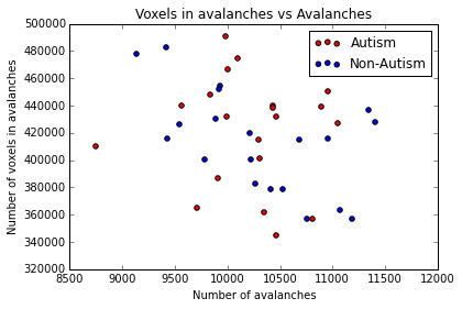
As example, here we show a small analysis between 2 groups of 21 subjects (autism and non-autism patients). The number of avalanches and the number of voxels belonging to an avalanche calculated after 2 neighbour clustering have been studied:

Means over groups and the ratio voxel_number per avalanche were also calculated over groups and differences were neither appreciate. More analyses had to be done, like computing the average lifetime of an avalanche and the avalanche-wise size.

Last week’s objectives

Our objectives for the last week are:

• Make last corrections and finalize documentation work as far as possible. In this task, we are going through the code to make insertions that would describe links between measures, graphics of interests, etc

• Evaluate the work done. Achievements / Fails as to create a little memorandum for the delivery, and possible lines for collaboration

• Pack the code and submit, in agreement with John and hoping to get impressions too

• Close project, open future: Make the toolbox more fruitful and better suited. Keep a line of communication for helping on further developments and distend chat about future ideas, and thank so much the team for accommodating us!

This week, as planned from the previous one, the integration has been extensively worked: the cpac_pipeline.py has now our workflow fully integrated and I have change the workflows into a single one, making it easier the call to the methods. Also, the treatment of the inputs has changed, since we are not making the extraction of the series anymore (another module of C-PAC is taking the responsibility). But more interestingly, we have enforced the Criticality package with the correction of the Point Process and Conditional Rate Mapping from the previous week and the developing of 2 new functions: Clustering and Avalanche detection algorithms.

For this algorithms, we have also followed the headlines explained in the paper of Tagliazucchi et al (“Criticality in large-scale brain fMRI dynamics unveiled by a novel point process analysis”), we have been able to extract Avalanches in the brain, wich opens a new perspective in the analysis of brain dynamics in C-PAC.

Clustering Detection

The technique is described, extracted from the section Methods of the paper, as:

To detect contiguous clusters of activated voxels (defined as those crossing the threshold), for each time step, the problem was reduced to the detection of connected components in a suitably defined graph or network. More precisely, for each volume, a graph was constructed having each voxel as a node, and two nodes connected with a link if they were both activated (BOLD signal above 1 SD) and also first neighbors in the spatial sense. The connected components of this graph correspond to clusters of contiguous activated voxels isolated from other similarly defined clusters.

The implementation of this approach was straightforward, but it has many checks to do, so it is an algorithm to code very carefully. It is a first draft of the algorithm and the purpose was to have a functional procedure asap. In future revisions, I will try to rewrite it in a more “pythonic way”.

1
2
3
4
5
6
7
8
9
10
11
12
13
14
15
16
17
18
19
20
21
22
23
24
25
26
27
28
29
30
31
32
33
34
35
36
37
38
39
40
41
42
43
44
45
46
47
48
49
50
51
52
53
54
55
56
57
58
59
60
61
62
63
64
65
66
67
68
69
70
71
72
73
74
75
76
77
78
79
80

# Detects clusters after Point Processing a Brain 
def cluster_detection(in_file):

    import numpy as np
    import os
    import nibabel as nb
    from CPAC.criticallity import point_process

    # Treat fMRI image
    img = nb.load(in_file)
    data = img.get_data()
    (n_x, n_y, n_z, n_t) = data.shape

    # Get the PP data
    pp_data = np.zeros((n_x, n_y, n_z, n_t))
    for i_ in range(n_x):
        for j_ in range(n_y):
            for k_ in range(n_z):
                voxel_data = data[i_,j_,k_,:]
                pp_data[i_,j_,k_,:] = point_process(voxel_data)

    cluster_graph_data_total = np.zeros((n_x, n_y, n_z, n_t))
    for t_ in range(n_t):
        time_slice = pp_data[:,:,:,t_]
        cluster_graph_data = np.zeros((n_x, n_y, n_z))
        cluster_number = 1

        for i_ in range(n_x):
            for j_ in range(n_y):
                for k_ in range(n_z):

                    if time_slice[i_,j_,k_] == 1: # is active, check if it has active neighboours
                        if time_slice[i_-1,j_,k_] or time_slice[i_+1,j_,k_] \
                        or time_slice[i_,j_-1,k_] or time_slice[i_,j_+1,k_] \
                        or time_slice[i_,j_,k_-1] or time_slice[i_,j_,k_+1]:

                            if cluster_graph_data[i_,j_,k_] == 0: # if is not in any previous cluster
                                this_cluster = (cluster_graph_data[i_-1,j_,k_] or cluster_graph_data[i_+1,j_,k_] \
                                or cluster_graph_data[i_,j_-1,k_] or cluster_graph_data[i_,j_+1,k_] \
                                or cluster_graph_data[i_,j_,k_-1] or cluster_graph_data[i_,j_,k_+1])

                                if this_cluster == 0: #no neighbours in any previous cluster neither
                                    this_cluster = cluster_number
                                    cluster_graph_data[i_,j_,k_] = this_cluster
                                    cluster_number = cluster_number + 1
                                else:
                                    #check cluster union
                                    merge_clusters = np.unique([cluster_graph_data[i_-1,j_,k_], cluster_graph_data[i_+1,j_,k_] \
                                , cluster_graph_data[i_,j_-1,k_], cluster_graph_data[i_,j_+1,k_] \
                                , cluster_graph_data[i_,j_,k_-1], cluster_graph_data[i_,j_,k_+1]])
                                    merge_clusters = merge_clusters[1:] #quit first value = 0

                                    this_cluster = merge_clusters[0]
                                    cluster_graph_data[i_,j_,k_] = this_cluster
                                    for cluster_to_merge in merge_clusters[1:]:
                                        cluster_graph_data[cluster_graph_data == cluster_to_merge] = this_cluster


                            else:
                                this_cluster = cluster_graph_data[i_,j_,k_]

                            #find neighbours and give cluster_number
                            if time_slice[i_-1,j_,k_] == 1:
                                cluster_graph_data[i_-1,j_,k_] = this_cluster
                            elif time_slice[i_+1,j_,k_] == 1:
                                cluster_graph_data[i_+1,j_,k_] = this_cluster
                            elif time_slice[i_,j_-1,k_] == 1:
                                cluster_graph_data[i_,j_-1,k_] = this_cluster
                            elif time_slice[i_,j_+1,k_] == 1:
                                cluster_graph_data[i_,j_+1,k_] = this_cluster
                            elif time_slice[i_,j_,k_-1] == 1:
                                cluster_graph_data[i_,j_,k_-1] = this_cluster
                            elif time_slice[i_,j_,k_+1] == 1:

                    # if not == 1¡, keep the search 
                        # if not neighbours, keep the search

        cluster_graph_data_total[:,:,:,t_] = cluster_graph_data

    return cluster_graph_data_total

Avalanche Detection

The technique can be easily described, extracted from the section Methods of the paper:

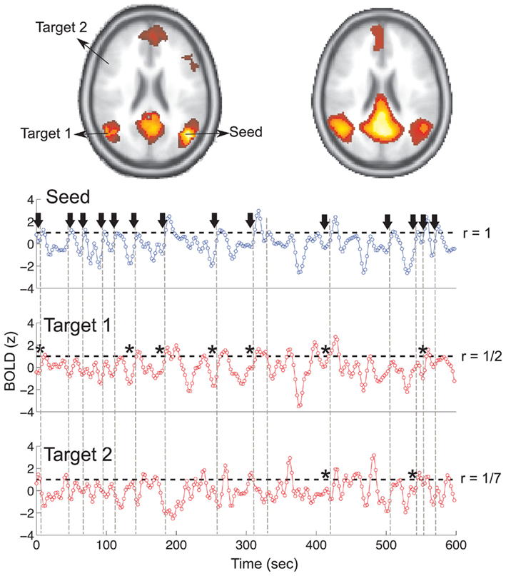
The point process is defined by the sequences of time points at which the BOLD signal crosses a given threshold from below. (…) To construct the conditional rates the point process is defined at a seed location and at the targets throughout the entire brain. The BOLD signal is extracted from a seed region (top trace) and the points (arrows and vertical dashed lines) are defined by the crossings at 1 SD (horizontal dashed lines). Every time the signal at a target region crosses the threshold (asterisks) up to 2 time steps later than in the seed, the rate at the target is increased in one unit. This rate is normalized by the number of points in the seed. The top panel shows the location of the seed and of the two example targets, as well as the resulting average conditional rates maps (left) and DMN obtained from PICA (right). Medium panels show the BOLD signal at the seed and at the two example target regions.

1
2
3
4
5
6
7
8
9
10
11
12
13
14
15
16
17
18
19
20
21
22
23
24
25
26
27
28
29
30
31
32
33
34
35
36
37
38
39
40
41
42
43
44
45
46
47
48
49
50
51
52
53
54
55
56
57
58
59
60
61
62
63
64
65
66
67
68
69
70
71
72
73
74
75
76
77
78
79

def avalanche_detec(cluster_file):

    import numpy as np
    import nibabel as nb
    import os

    # Treat fMRI image
    img = nb.load(cluster_file)
    cluster_data = img.get_data()
    (n_x, n_y, n_z, n_t) = cluster_data.shape

    avalanche_id_total = np.zeros((n_x, n_y, n_z, n_t))
    avalanche_id_num = 1

    for t_ in range(n_t):

        if t_ == 0: #if first timestep, all are candidates
            time_slice = cluster_data[:,:,:,t_]
            time_slice_fut = cluster_data[:,:,:,t_+1]

            avalanche_id_now = avalanche_id_total[:,:,:,t_]
            avalanche_id_fut = avalanche_id_total[:,:,:,t_+1]

            for cluster in np.unique(cluster_data[:,:,:,t_])[1:]: #iterate over clusters
                # NEW AVALANCHE CASE
                if np.count_nonzero(time_slice_fut[(time_slice==cluster)]) >= 1 :
                    avalanche_id_now[(time_slice==cluster)] = avalanche_id_num

                    for value in np.unique(time_slice_fut[(time_slice==cluster)])[1:]:
                        avalanche_id_fut[(time_slice_fut==value)] = avalanche_id_num

                    avalanche_id_num = avalanche_id_num +1

                    avalanche_id_total[:,:,:,t_] = avalanche_id_now
                    avalanche_id_total[:,:,:,t_+1] = avalanche_id_fut


        elif t_ < (n_t-1):  #if not first timestep, check previous
            print t_
            #time_slice_past = cluster_data[:,:,:,t_-1]
            time_slice = cluster_data[:,:,:,t_]
            time_slice_fut = cluster_data[:,:,:,t_+1]

            avalanche_id_now = avalanche_id_total[:,:,:,t_]
            avalanche_id_fut = avalanche_id_total[:,:,:,t_+1]

            for cluster in np.unique(cluster_data[:,:,:,t_])[1:]:
                # PREVIOUS AVALANCHE CASE
                if np.count_nonzero(avalanche_id_now[(time_slice==cluster)]) != 0:
                    if np.count_nonzero(time_slice_fut[(time_slice==cluster)]) >= 1 :

                        this_avalanche = avalanche_id_now[(time_slice==cluster)][0]

                        for value in np.unique(time_slice_fut[(time_slice==cluster)])[1:]:
                            avalanche_id_fut[(time_slice_fut==value)] = this_avalanche

                        avalanche_id_total[:,:,:,t_+1] = avalanche_id_fut

                # NEW AVALANCHE CASE
                elif np.count_nonzero(avalanche_id_now[(time_slice==cluster)]) == 0: #and np.count_nonzero(time_slice_past[(time_slice==cluster)]) == 0:
                    if np.count_nonzero(time_slice_fut[(time_slice==cluster)]) >= 1 :

                        avalanche_id_now[(time_slice==cluster)] = avalanche_id_num

                        for value in np.unique(time_slice_fut[(time_slice==cluster)])[1:]:
                            avalanche_id_fut[(time_slice_fut==value)] = avalanche_id_num

                        avalanche_id_num = avalanche_id_num + 1

                        avalanche_id_total[:,:,:,t_] = avalanche_id_now
                        avalanche_id_total[:,:,:,t_+1] = avalanche_id_fut


    img_new = nb.Nifti1Image(avalanche_id_total, header=img.get_header(), affine=img.get_affine())
    # Reconstruct the 4D volume
    cond_rm_file = os.path.join(os.getcwd(), 'avalanche.nii.gz')
    img_new.to_filename(cond_rm_file)

    return avalanche_id_total

Discussions on Clustering and Avalanche detection

Clustering Detection

After coding the algorithms as explained in the paper, we extended it to some discussion, we found further questions of interest with regard to the algorithm. Questions that have emerged after initial implementation are the following:

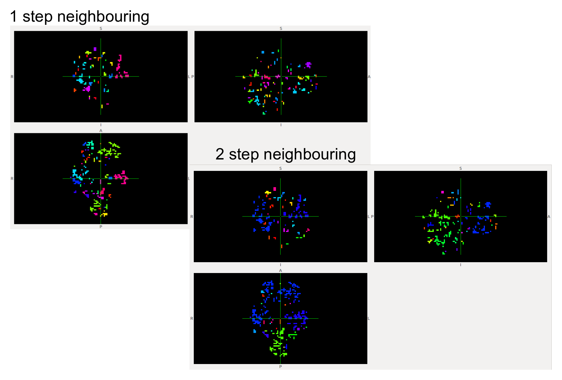
I was wondering about the root aspects of defining 1 single neighbour and not more in the clustering detection and also about the decision of determining a cluster just from one neighbouring. Which are the implications of these assumptions? I actually tried the implementation extending the neighbouring adding more neighbours (2 and 3).

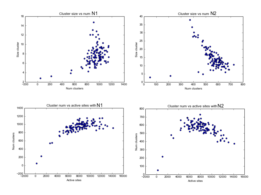
I came across with less and bigger clusters, which we discussed for its possible interest specifically with brain images. See images below for clusters with the proposed 1 distance for neighbours and with a distance of 2, at a given time:

From these approaches we can have some statistics, showing that the choice of the number of neighbours to consider is not a trivial decision:

Avalanche Detection

We collected all the avalanches for a given subject in a 4D Nifti file. Avalanches were significantly different depending of the choice of the neighbouring size (due to the change of the size of the mean cluster). Here we show a first approximation, we would have liked to make a movie, but we ran out of time for this week.

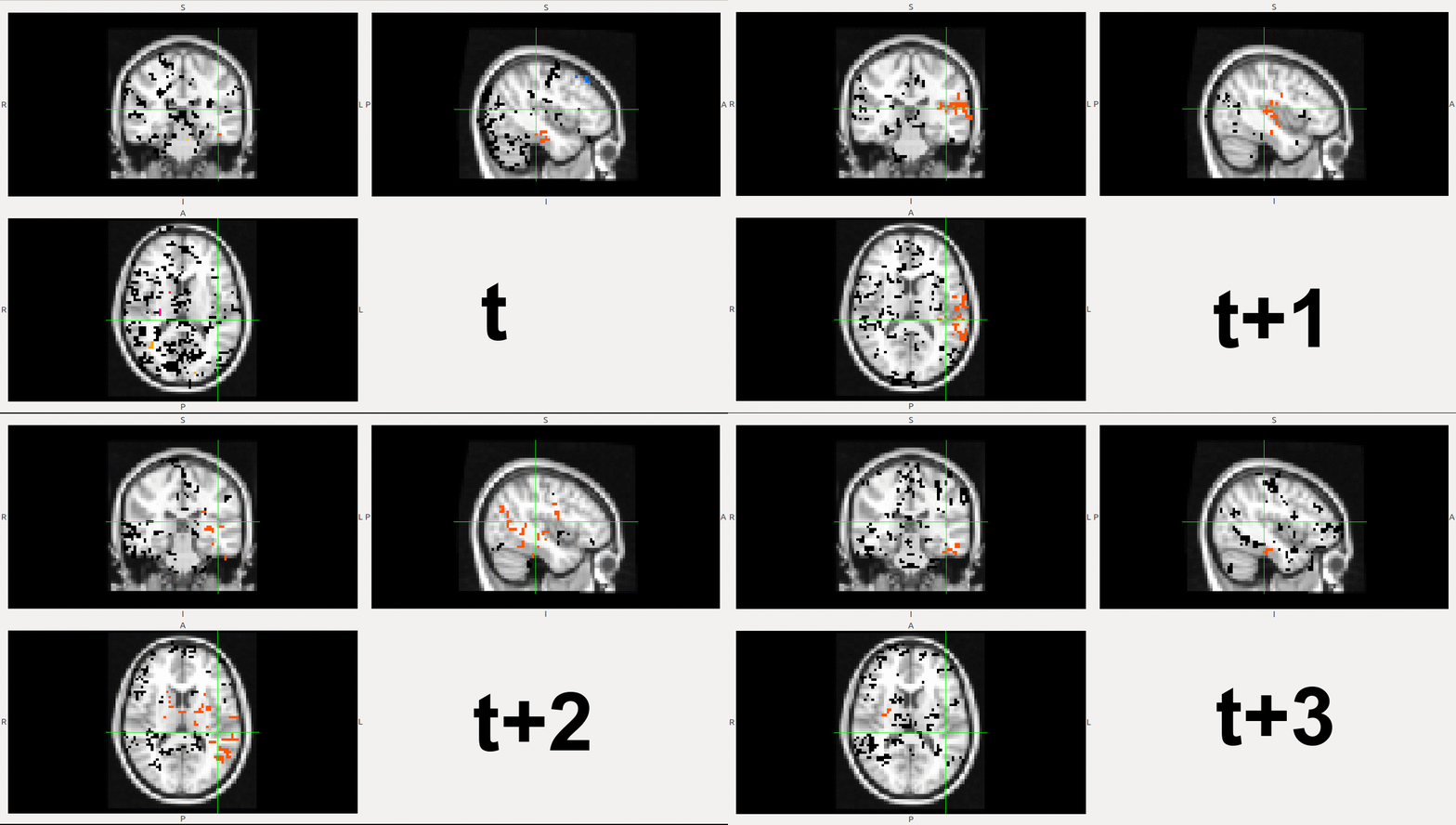
Here I have made a gif to represent how an avalanche is. This is an avalanche for the N2 cluster, take into account just the voxels in red/orange. It can be showed how the avalanche borns, grows and spreads, and finally dies.

Heading last week of coding

Our objectives for next week are:

• Perform extensive testing over the measures and chose which ones are going to be in the package.

• Make code corrections and comment all the measures. This will head us into the documentation we have to make.

We are heading the end of the quarter and our toolbox is starting to be mature, while we investigate the many links and uses between tools. This week we have gone through important steps (but at the same time ongoing discussions due to the rich materials produced at this stage). Two main new things we have done, beyond the polishing of previous tools and validating ongoing:

• The integration of the toolbox in CPAC’s pipeline is almost complete. This has been a tough task to do, since the internals of CPAC are quite large, with many flows and structures, but the main idea is clear: The work to do is to link the inputs you get from the GUI and the data already calculated previously in other CPAC’s modules with your workflows inputs and integrate them in the main pipeline.

• Point Process Analysis and Conditional Rate Maps calculation: Following the initial plan, we have developed some new methods to test the time scale side of the toolbox and while Supraja is progressing with multifractal analysis in parallel.

Following the instructions in the paper of Tagliazucchi et al (“Criticality in large-scale brain fMRI dynamics unveiled by a novel point process analysis”), we have been able to code the base point process approach followed of a Conditional Rate Map building as in the paper.

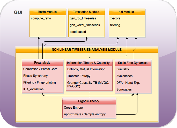
And last, in terms of toolbox integration, new cross relationships have been looked at. Some of those are portrayed from our last model:

Integration of the toolbox in CPAC’s pipeline

After carefully having explored the main pipeline, we realized that in order to not to repeat code and structures that are already developed, I had to make some changes in my initial workflows. At the beginning of the project, I coded them as independent workflows, with independent behaviour and inputs, and some helper functions that are already integrated in CPAC but that where necessary for me in that moment. Now, I have to link the data that would be already in CPAC, change the treatment of the inputs of my workflows and integrate them as a single tool.

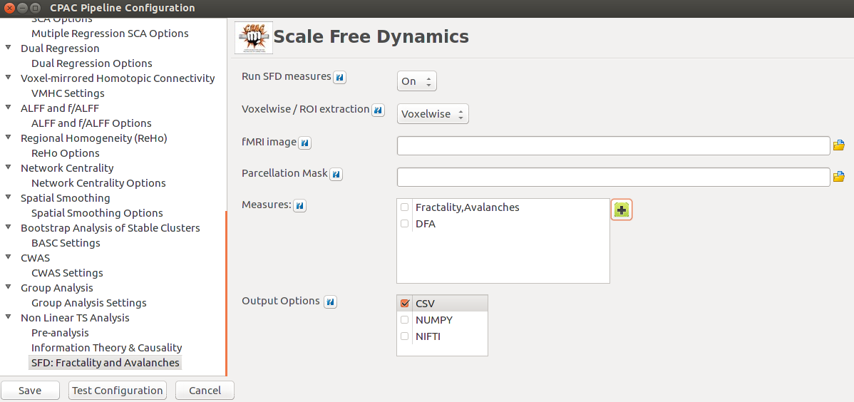
That will have effect too in the configuration of the GUI I proposed two weeks ago, being now more efficient. We have now all measures in a joint page of the GUI, having separated each of the main boxes of the initial plan in three different checkboxes with a common input. Also, the input data for my workflows will come from the TSE module of CPAC, which already makes these extractions. I have to modify my functions to work with 1D files (I have already the main code block built, since I already treated with this data type in the analysis of the 400 regions).

In the main pipeline, I have inserted the NLTSA workflow:

https://github.com/roijo/C-PAC_complexitytools/blob/master/CPAC/pipeline/cpac_pipeline.py#L3207-L3368

It can be seen in the code that still are many things to change and improve, I am receiving crucial help from developers, to fully understand how the main pipeline works and transferring this knowledge to all discussions.

The main structure at the moment, is a three block structure as previously proposed, plus the insert of qualities that measures derived from ergodic theory rely on. From these, I let the user to choose which one of them (the measures inside each of them) to calculate. I will change my workflows (I will have one per measure-box) and inside them, the measures will be called directly depending if they have been chosen by the user or not.

Point Process Analysis and Conditional Rate Maps

The technique can be easily described, extracted from the section Methods of the paper:

The point process is defined by the sequences of time points at which the BOLD signal crosses a given threshold from below. (…) To construct the conditional rates the point process is defined at a seed location and at the targets throughout the entire brain. The BOLD signal is extracted from a seed region (top trace) and the points (arrows and vertical dashed lines) are defined by the crossings at 1 SD (horizontal dashed lines). Every time the signal at a target region crosses the threshold (asterisks) up to 2 time steps later than in the seed, the rate at the target is increased in one unit. This rate is normalized by the number of points in the seed. The top panel shows the location of the seed and of the two example targets, as well as the resulting average conditional rates maps (left) and DMN obtained from PICA (right). Medium panels show the BOLD signal at the seed and at the two example target regions.

From that explanation a pair of functions have been developed:

1
2
3
4
5
6
7
8
9
10
11
12

# Point process analysis for a signal. Values equal to 1 when the original value 
# is higher than the threshold (1*SD)
def point_process(signal):

    import numpy as np

    pp_signal = np.zeros(signal.shape[0])
    th = np.std(signal)

    pp_signal[signal > th] = 1

    return pp_signal

1
2
3
4
5
6
7
8
9
10
11
12
13
14
15
16
17
18
19
20
21
22
23
24
25
26
27
28
29
30
31
32
33
34
35
36

# Conditional Rate Map. Given an fMRI, extract timeseries, calculate Point Process
# and then the Rate Map for each voxel given a seed   
def cond_rm(in_file, seed_location):

    import numpy as np
    import os
    import nibabel as nb

    # Treat fMRI image
    img = nb.load(in_file)
    #print img.shape
    data = img.get_data()

    (n_x, n_y, n_z, n_t) = data.shape

    K = np.zeros((n_x, n_y, n_z))
    # Extract seed and pp
    seed_data = data[seed_location[0], seed_location[1], seed_location[2],:]
    pp_seed_data = point_process(seed_data)
    r = np.count_nonzero(pp_seed_data)
    # Calculate each PP signal
    for i_ in range(n_x):
        for j_ in range(n_y):
            for k_ in range(n_z):

                target_data = data[i_,j_,k_,:]
                pp_target_data = point_process(target_data)

                # LOGIC AND (target/seed) and count(signal == 1), that will give you the X/r parameter [0,1]
                K[i_,j_,k_] = np.count_nonzero(np.logical_and(pp_seed_data,pp_target_data))/float(r)

    # Reconstruct the 3D volume
    cond_rm_file = os.path.join(os.getcwd(), 'cond_rm.nii.gz')
    img.to_filename(cond_rm_file)

    return cond_rm_file

As it can be seen, there is still a small change to be done in the CRM function. As described in the paper, the target point processed signal has to be checked in the same time point as the seed and up to 2 time steps later. As it can be derived from the image, is takes all the values crossing the threshold in a row just as one crossing. I would like to keep my function in a pythonic way and I don’t find a way of computing the CRM without messing everything up with index checking to satisfy the requirements of the algorithm. Also, it would be desirable to know if the data already satisfies the requirements of z-scoring and HRF deconvolution as proposed in the paper and if this has effect on the algorithm results.

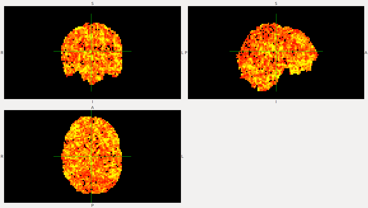
From these calculations, we can start extracting volumes such as:

We are now discussing about the possibility of following the analysis by building the Clustering and the Avalanche detection, but they are not as well described in the paper and we have to make a evaluation of the time we have to finish the project.

Relation between Correlation and CMR’s number of point-wise events

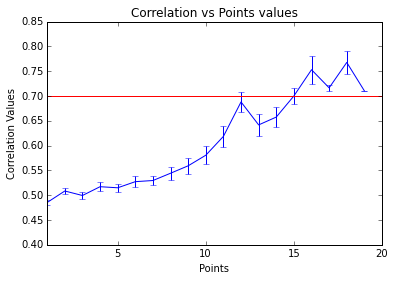
To make a comparison between the number of points that are necessary to reach a specific information level with the point process algorithm, we have used the correlation to identify highly synchronized timeseries. What we have done here is to build a relation between the synchrony of two variables and the point peaks that share each other after point processing them (CMR without normalizing).

As an initial optimization we can find to which level point process transients can be translated to a point of criticality. This analysis has been produced at the voxel-wise level from ABIDE subjects, properly checked and preprocessed. Here, we can see how the increasing of the (mean) synchrony between two variables, increases the points that they share. This is a really nice finding, because it shows how point process can describe the change of regime associated with functional connectivity.

We can observe how once reached a threshold of 0.7 correlation point-processes can saturate giving a new quality to connectivity between regions.

Others

• Even if the VAR model calculation was corrected in the previous week, there was still an issue with the calculation of pwcgc() , the internal loop has been already corrected. We have tested the function over data and looks to have the same performance as the original Matlab function. Different distributions of these will be last discussed if we can define more optimal models.

• We have been discussing about the need of visualization of some analysis inside and some statistics CPAC (Pandas integration) . This is maybe a sore point that would be better to discuss with main developers.

• Next week we will follow our work with the integration, enforcement of criticality package and also we are into final integration of all our measures (phase measures integration with Scale Free Dynamics ones like DFA/Hurst exponent, for example).

We are trying to converge to an easy and clear design of the GUI of our toolbox that integrates in CPAC’s structure and allows users to use it. We are trying here to avoid redundant options in the workflow and it is becoming a quite difficult task, since we want the measures to be separated in differentiated subgroups, but at the same time, give the toolbox the possibility of using common functions (such as the extraction of the timeseries). It has to be non-redundant in this way, the most complicated thing will be the correct use of data structures (to take the ones that are already being generated from other modules in CPAC and to check if the series of a volume had been already extracted, in order to do not duplicate efforts). The design has to be generalizable enough that it can be used in other workflows.

Planning of the GUI for NLTSA module

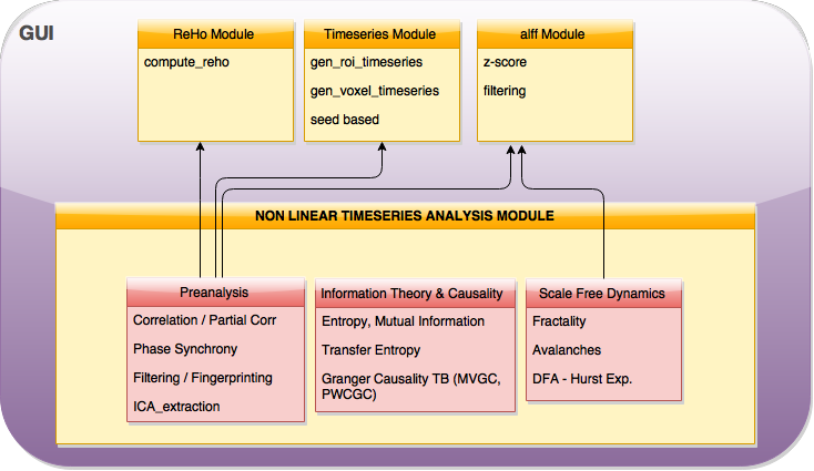
As the most important part of developing new software, it is always necessary to have a good developing plan. For the purpose of building the GUI for our toolbox, we have divided all our measures in 3 main groups:

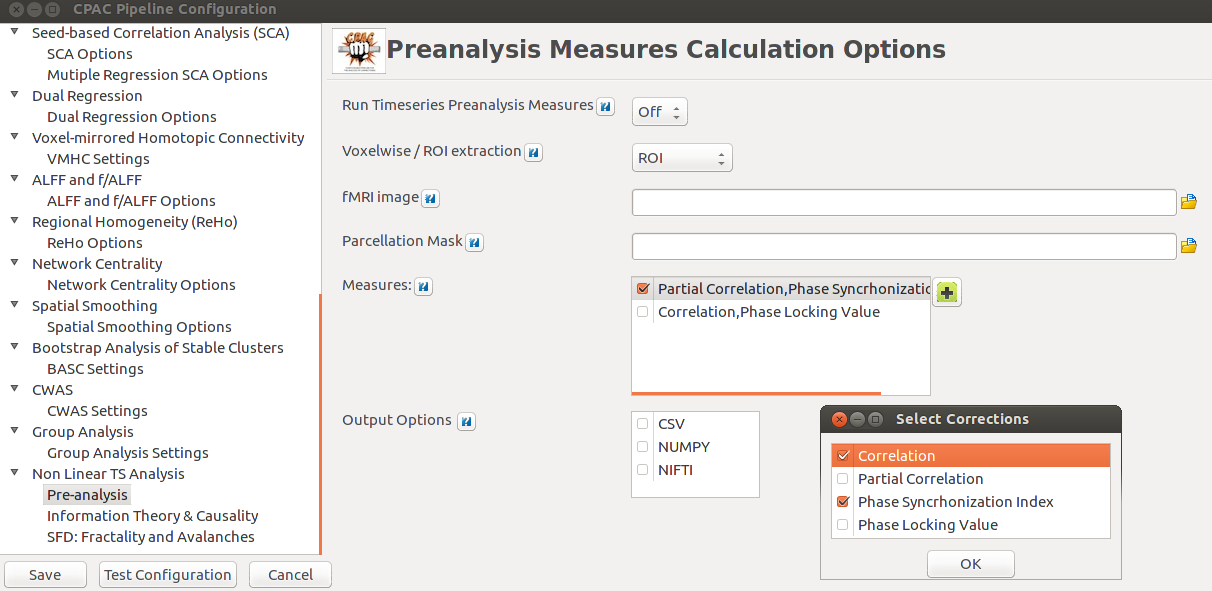
• Pre-Analysis measures: The ones that not correspond directly to NonLinearTimeSeriesAnalysis and can be applied directly into the extracted data. We can find here synchrony measures in time (correlation, partial correlation) and frequency domain (phase synchrony index, phase locking value). Also, treatment of fingerprints and ICA timeseries extraction are due to be added in this submodule.
• Information Theory and Causality measures: The ones coming from the informative framework and causality. These measures involve the acquisition of information flow and sharing between variables (Mutual Information, Transfer Entropy, Granger Causality Toolbox measures (MVGC, PWCGC)).
• Scale free dynamics measures: This is the box that make use of the most advanced measures (fractality, avalanches, detrended fluctuation analysis, Hurst exponents). These measures are still pending of being developed (planned for August), so we have still not decided about the inputs and the outputs they are generating.

The schema shown above has been resumed in the next diagram. Most of the modules make use of other modules functions (we have tried to not being redundant with CPAC’s code). We have ensured that the helper functions developed for our toolbox are available also from outside our module.

Implementation of the GUI

Following the instructions published in the previous post, there has been straightforward to build up the 3 subgroups, as they are quite similar between each other. The most important feature for us was the possibility of calculating the measures independently (there is no need of calculating all of them, the user can choose whether to apply the different measures without restriction).

A serious work must be done in flow-controlling inside cpac_pipeline.py to avoid repeating the operations present in the submodules (mainly, timeseries generation. Once that are generated, there is no point in extracting them again). Also, it is important to have well connected the toolbox to the main CPAC’s workflow and check whether the data has been previously extracted. Maybe we can talk at some point soon about this and listen to developers thoughts, comments in the post will be very welcomed. Also, we left the door open for interesting modifications that could happen (the 3rd submodule is still pending of being coded and we have in mind to deal with visualization and data presentation). The whole integration will be held in the last week of GSoC with the help of all collaborators and students.

Synchrony measures in ADHD data

As we are trying not to evaluate all our measures together at the end, this week we have tried extensively our new dataset from ADHD200 (specific information about the dataset and how we did our first experiment in previous post ).

We had two measures to test over this data, “phase synchrony index” (which is a self-informative value about the synchrony level of a specific signal) and “phase locking value” (which is the relation between the synchronicity of 2 variables).

We had two measures to test over this data, “phase synchrony index” or PSI (which is a self-informative value about the synchrony level of a specific signal) and “phase locking value” or PLV (which is the relation between the synchronicity of 2 variables).

Results

The PSI is a single variable measure, so it is just an self-informative measure. First results showed that the data extracted with the cc400 and cc1000 parcellations had a low synchrony level (some of them looked totally desynchronized). Overall, there was not much to say about differences between ADHD patients and controls.

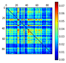
The PLV, however, showed that the synchrony between some of the signals was strong (>0.7). As these parcellations are randomly created and assigned, consecutive ROIs have not spatial relation and showing the usual matrixes was not going to be informative.

Solved GC VAR model calculation

We have changed the paradigm of measuring the residuals for the Granger Causality calculation. Instead of calculating the covariance matrix of the data, which was creating problems later with the VAR model, we have change this. Now, the residuals are calculated directly from the data (the regression model used was OLS using QR decomposition. Specifications in MVGC toolbox docs), without performing the calculation of the covariance matrix.

We performed a small evaluation of the PWGC over our ADHD200 dataset and results were not visually different between groups. We are working in an appropriate way of showing results coming from these measures.

This week I have been trying to work with the migration of our modules to the GUI. For that, you will need to perform three main steps:

• Create the interface for your modules (2 steps)
  • Define your space in the main configuration window tree. (Name your module/submodules)
  • Define a window with configuration options (inputs and output of your workflow basically) for each one of your modules/submodules. The main window of the module usually is referred to an html file explaining what this module does and how does it work.
• Link the GUI with your workflows (1 step)
  • Link the configuration window of each of the submodules with the corresponding workflow through the pipeline module, allowing the execution of your workflows.

Create the interface for your modules

STEP 1

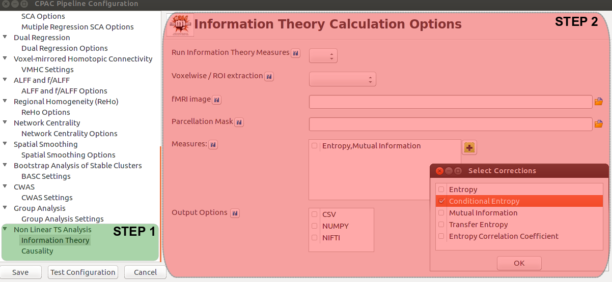
The interface for the modules needs to be created. This is done by adding your module structure to the main configuration tree (a bit of planification is needed before deciding how the module structure is going to be organized). The first 2 steps should be done in parallel, I choosed to create the tree structure first, because I thought it was better a up to bottom approach.

First of all, you have to define your space in the config_window file, in the Class named ‘Mybook’.

There, you can find all the module names that will be listed in the main left of the pipeline configuration window. As an example, I have added some lines at the end of the Class:

1
2
3
4
5
6
7
8
9

   self.AddPage(page43, "CWAS", wx.ID_ANY)
        self.AddSubPage(page44, "CWAS Settings", wx.ID_ANY)

        self.AddPage(page45, "Group Analysis", wx.ID_ANY)
        self.AddSubPage(page46, "Group Analysis Settings", wx.ID_ANY)
        ### ADDED NEXT 3 LINES: 48 is my main module name. 49 and 50 submodules inside 48
        self.AddPage(page48, "Non Linear TS Analysis", wx.ID_ANY)
        self.AddSubPage(page49, "Information Theory", wx.ID_ANY)
        self.AddSubPage(page50, "Causality", wx.ID_ANY)

It is also important to add the name of your GUI Classes in the import at the beginning of the file. In the second step, these Classes will be defined.

STEP 2

In this step the Classes that create your configuration pages must be created. Here, it will be defined a window with configuration options (inputs and output of your workflow basically) for each one of your modules/submodules. For this purpose, it is neccessary to create a new file in the ‘pages’ directory, other files can be used an example.

The main window of the module (in our example the 48) is usually referred to an html file explaining what this module does and how does it work. If you don’t have such file yet, you can leave it blank. For the rest of submodules, as CPAC’s has its own framework built over wx, we can choose between many specific buttons and data tpyes to add to our window:

1
2
3
4
5
6
7
8
9
10
11
12
13
14
15
16
17
18
19
20

control = enum(CHOICE_BOX = 0,
               TEXT_BOX = 1,
               COMBO_BOX = 2,
               INT_CTRL = 3,
               FLOAT_CTRL = 4,
               DIR_COMBO_BOX = 5,
               CHECKLIST_BOX = 6,
               LISTBOX_COMBO = 7,
               TEXTBOX_COMBO = 8,
               CHECKBOX_GRID = 9)

dtype = enum(BOOL = 0,
             STR= 1,
             NUM= 2,
             LBOOL = 3,
             LSTR = 4,
             LNUM = 5,
             LOFL = 6,
             COMBO = 7,
             LDICT= 8 )

This is an example of how it can be a GUI frame for our toolbox:

1
2
3
4
5
6
7
8
9
10
11
12
13
14
15
16
17
18
19
20
21
22
23
24
25
26
27
28
29
30
31
32
33
34
35
36
37
38
39
40
41
42
43
44
45
46
47
48
49
50
51
52
53
54
55
56
57
58
59

class InformationTheory(wx.ScrolledWindow):

    def __init__(self, parent, counter = 0):
        wx.ScrolledWindow.__init__(self, parent)
        self.counter = counter

        self.page = GenericClass(self, "Information Theory Calculation Options")

        self.page.add(label="Run Information Theory Measures",
                 control=control.CHOICE_BOX,
                 name='runIT',
                 type=dtype.LSTR,
                 comment="Run Information Theory Measures",
                 values=["Off","On"],
                 wkf_switch = True)

        self.page.add(label="Voxelwise / ROI extraction",
                 control=control.CHOICE_BOX,
                 name='voxel_roi',
                 type=dtype.LSTR,
                 comment="Run Information Theory Measures voxelwise or after ROI timeseries             extraction", values=["Voxelwise","ROI","Voxelwise/ROI"],
                 wkf_switch = True)

        self.page.add(label="fMRI image",
                     control=control.COMBO_BOX,
                     name='input_image',
                     type=dtype.STR,
                     comment="fMRI image for calculation")

        self.page.add(label="Parcellation Mask",
                     control=control.COMBO_BOX,
                     name='input_mask',
                     type=dtype.STR,
                     comment="Parcellation Mask if you want to calculate")

        self.page.add(label = "Measures:",
                      #control = control.CHECKLISTBOX_COMBO,
                      control = control.LISTBOX_COMBO,
                      name = "Measures",
                      type = dtype.LDICT,
                      values = ['Entropy', 'Conditional Entropy','Mutual Information','Transfer Entropy','Entropy Correlation Coefficient'],
                      comment = "Select which IT measures to apply:\n"\
                                "ent = Entropy\n"\
                                 "condent = Conditional Entropy\n"\
                                 "mi = Mutual Information\n"\
                                 "te = Transfer Entropy\n"\
                                 "ecc = Entropy Correlation Coefficient\n",
                     size = (300,120),
                     combo_type =1)

        self.page.add(label="Output Options ",
                      control=control.CHECKLIST_BOX,
                      name="measure_options",
                      type=dtype.LBOOL,
                      values=['CSV', 'NUMPY','NIFTI'],
                      comment="By default, results are written as NIFTI files. Additional output formats are as a .csv spreadsheet or a Numpy array.")

        self.page.set_sizer()
        parent.get_page_list().append(self)

It is important to update the init file of the folder ‘pages’ to make the new file available and checking all the intermodule dependencies and imports. After doing these modifications, the modifications will be seen as long as the MainUI file runs without problem.

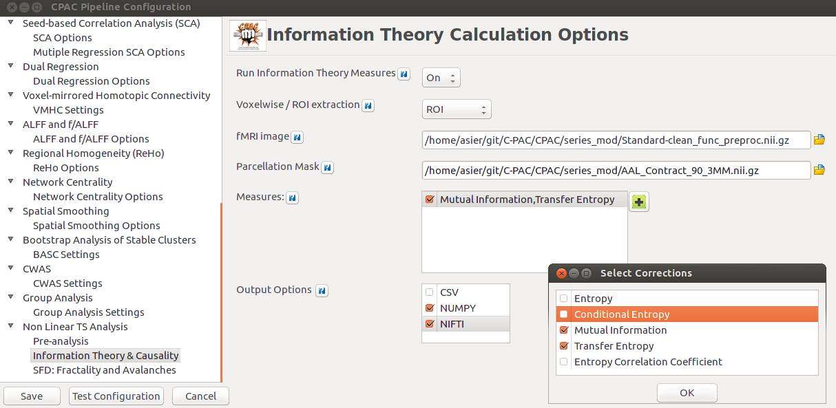
In the next figure, it can be seen how the example code is translated into the GUI:

After completing your configuration, a YAML file will be created with the information provided into the different inputs.

Link the GUI with your workflows

STEP 3

This is probably the most important step along with having a good planification of the needs of the module. The objective here is to link the configuration window of each of the submodules with the corresponding workflow through the pipeline module and specifically the cpac_pipeline file, allowing the execution of your workflows.

First of all, it is needed to import the workflows into the file. After that, and having as a reference other workflow insertions, you can take the input data saved in the previous step from a Configuration object called ‘c’. This ‘c’ variable is an abstract representation used to store the options for the pipeline configuration YAML. The use of the YAML file, allows users to load preconfigured files easily. The YAML was generated by the GUI in the previous step and it is reloaded back in by cpac_runner as a Configuration object (‘c’). Finally, cpac_runner.py passes the Configuration object to cpac_pipeline.py as an argument.

There is the need of checking if the inputs are correct (otherwise, raise an error message), create the workflow and give to it the inputs extracted from ‘c’. cpac_pipeline.py is where the Nipype workflow object for each pipeline strategy is constructed via flow control. We will want to add a code block similar to this in order to add the nonlinear time-series node to these workflows. The functions will be encapsulated within nodes and connected to a workflow.

Short example of how to manage the inputs:

1
2
3
4
5
6
7
8
9
10
11
12
13
14
15
16
17
18
19
20

    '''
    Inserting NLTSA
    Workflow
    '''

    new_strat_list = []
    num_strat = 0

    if 1 in c.runIT:
        for strat in strat_list:

  if 'mi' in c.MEASURES

            pipeline = create_mi()
            pipeline.inputs.inputspec.in_file = c.input_image
            pipeline.inputs.inputspec.mask_file = c.input_mask
            pipeline.run()

            num_strat += 1
    strat_list += new_strat_list

After completing this last step, the new module of CPAC should be working.

This week we have been clarifying the issues involved on MVGC’s statistical model. Namely, the model to calculate the residuals that we use to measure the causality could be interpreted in a different way that we need to have well settled. Once we have identified the problem and clarified how this model should better be, we will shortly readdress and implement the experimentation done.

Testing on real datasets

We did our first systematic efforts to test workflows integrally with fMRI data and find if the results were coherent with the technique.

Materials and methods:

• Data was used from the ADHD200 initiative as recommended . For this purpose, I selected the preprocessed NeuroImage dataset (4mm voxel size).
• Data sampling: After having downloaded the data, we ruled out several subjects from the study (left handed…), resulting in 34 total subjects and then they were classified in 2 main groups: Controls and ADHD patients (20/14).
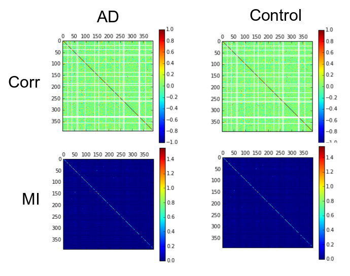
• Image processing: I extracted the mean timeseries of this data using the cc400 and cc1000 masks and performed a test analysis. Corr, TE and MI were computed over the series. Here I show resulting matrixes for the cc400 parcellation (results for cc1000 were similar).

First numbers showed than calculating the mean CC, TE and MI matrices for each group, most of the measures were close to 0. The results for the 1000 ROI parcellation was similar. This is a behaviour that it was also shown for the YALE preprocessed subsample (ABIDE) that we have been using in previous attempts for these high parcellated masks.

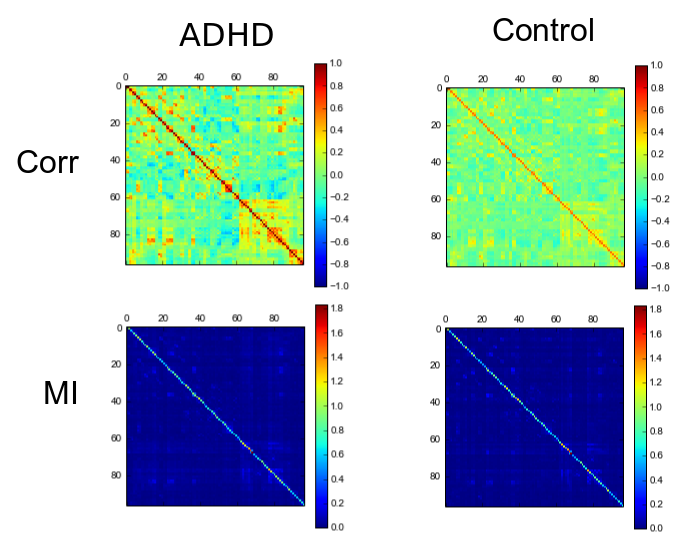
We tried a similar approach with the data already extracted for cc400 and TT parcellations and while cc400 showed same results as our self-extracted series (we can say that our extraction method works fine) the TT parcellated data showed the following structures:

One can visually appreciate slight changes in ADHD patients compared to controls. There is the need of further analyzing these results, but it is not the aim of this study. This result outlined the possibility that some parcellations are better suited for specific analyses, and that the ability of different ROI layouts to parcellate a brain, may impact on the capacity of extracting information from the dataset.

Being the calculation of the measures the same for 90, 400 and 1000 regions, I can just visually appreciate clear structures in the parcellation of 90 regions (which does not actually say much about the data, that should be furtherly analyzed). This could have a major reason in the way that different parcellation masks are created. The measures were also tested over the same data in Matlab having the same results to test wheter our methods were correct or not.

Repository and invitation to collaborate

It was an important moment for us to be able to start interact on Github for two main reasons. Firstly, to be able to discuss and comment in a more applied way and have this in a single repository that everyone included on the complexity toolboxes could access (included CMI!). And secondly to have a repository that deployed on our cluster allow us to process large datasets to validate and document. This repository has unified on:

https://github.com/roijo/C-PAC_complexitytools

Similarly, knowing well ADHD200 and ABIDE (CORR is also there) was a necessary task to do that we are doing in common.

Finally, I have added a slightly modificated function used in a previous work by Cameron, that saves the results into a Nifti file, making it easier to keep the results and export them.

As we have reached the midterm of the project, We are writing this post as a summary of what we have been working on and which are our next objectives. Our overall evaluation of our work is positive and we are excited about keep the coding and learning.

Theory and discussion

In one hand, we have been weekly discussing about the measures we had to implement, having debates about the information we could get from them and feasibility and practicality of these measures integrated in CPAC and in terms of development. Also, it has been a hard-work of researching and learning about new techniques and tools used in the field, linked not only to measures related to non-linear analysis of the series, but also to a wide variety of preprocessing techniques, optimization and python language learning. Our weekly discussions about data and integration of other imaging environments and other parts of CPAC (ie. FSL have been stimulating).

Coding

In the other hand, as a consequence of the previous point, we have accomplished the goal of implementing several measures, helper functions and tools building partially a toolbox for the analysis of non-linear information of series that will need triming and revision, on the principles of utility and complementarity. Organisation of these measures and outputs are also to come.

I have developed 4 working workflows of measures based on correlation and Information Theory between pairs of variables (Ivan has developed others complementing my work):

• Correlation WF
• Partial Correlation WF
• Mutual Information WF
• Transfer Entropy WF

Additionally, the toolbox has several measures and helper functions some more completed than others that we are polishing and comparing to select some as to include in the toolbox:

• Shannon entropy
• ApEn and SampEn (sampling entropies)
• Conditional entropies
• Entropy Correlation Coefficient
• Phase synchronization (as explained in my last entry)
• Phase Locking Values
• TE based in covariances for gaussian variables (no need of discretization).
• Entropy Correlation Coefficient
• Helper functions:
  • Voxel-wise timeseries generator from fMRI data
  • ROI timeseries generator from fMRI data
  • Transform (BIC discretization of signals based on Equiquantization criteria and discretization formalisms by Ivan)
  • Frequency filters and bands
  • Phase extractors

And also a Granger Causality (GC) module (Implementing Pairwise Conditional GC and MultiVariate GC using a VAR model) that still is under last testings and bug-correcting phase with the following functions that can be found in GitHub:

• Granger Causality functions based on VAR model:
  • tsdata_to_autocov: Timeseries to autocovariance matrix calculation
  • autocov_to_var: Calculation of the coefficients and the residuals using the VAR model.
  • autocov_to_pwcgc: Calculation of the Pairwise Granger Causality using the residuals previously calculated.
  • autocov_to_mvgc: Calculation of the Multivariate Granger Causality using the residuals previously calculated.

Testing over real data

Finally, there has been an application of the developed measures to real fMRI data, having reported some preliminary results. These results can be found in previous entries of this blog:

Correlation, Entropies and Mutual Information, Transfer Entropy and Phase Synchrony.

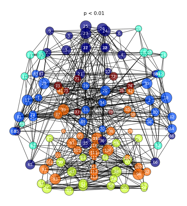
We are towards starting using extensively the NCoRR database for real data usage with the measures and establish the use of new atlases to extend the 90 ROIs that we have been working with to 512 or/and 1024 regions and voxel-wise for modelisation in our cluster. Also, we are dedicated to graphic representation and results for documentation. An basic idea idea of how we could represent our matrices using networkx capabilities is explained here as orientative, by taking correlation matrixes (could be any other measure’s bi-directional results matrix) and generating figures like these:

Next objectives

Even if we are successfully completing our initial plan, we have still work to do:

The obvious point is that testing these tools in real data and modelling them and their parameters for robustness and effective documentation, comparing also several situations and testing the code efficiency and stability.

Other practicalities I would like to point some TO-DO’s and objectives towards the second (and last) part of the project:

• Merging of both students repositories and having a copy of it in a cluster, allowing running studies on it.
• Solve code problems and developer strategies alike to CPAC already existing code (efficiency and some errors in measures).
• Work on the integration with CPAC (GUI building and dependencies).
• Keep following the initial plan: Cross-entropies, Fingerprints and Avalanche-point process modelisation. Discuss extensively about features to add, most relevant measures and future aplications over real data.
• Implement measures of multiscale dynamics .
• We have now a primitive and easy version of calculating the numbers of bins via Equantization. We are discussing more advanced methods to do it and it is likely to develop an alternative.
• Related to frecuencies (develop using what we already have as a base):
  • Implement Sample Entropies.
  • Fingerprints -> Determine important frequencies. Use of the power spectrum.

The Hilbert Transform is a linear operator which takes a function, u(t), and produces a function, H(u)(t), with the same domain.

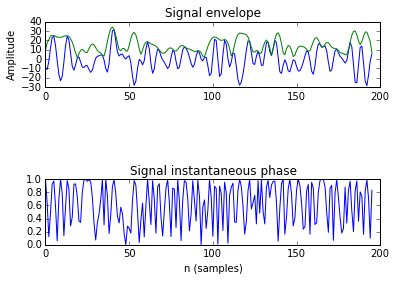
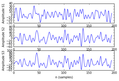
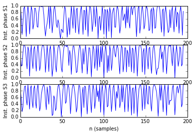
In python, we can compute the analytic signal, using the Hilbert transform. This analytic signal is used for many things, like computing the envelope of a signal or the instantaneous phase of the signal. Our calculation of the instantaneous phase is in the range [0,1], computed over the cos() function of the angle of the Hilbert Transform coefficients. We have choosen a random signal of an fMRI file to show the example:

1

env = numpy.abs(sigtool.hilbert(s))

1
2
3

ht = sigtool.hilbert(s)
px = np.angle(ht) # instantaneous phase
inst_p = np.sqrt((np.cos(px))**2) # modulus of the angle in [0,1]

With this instantaneous phase, we can code easyly the two functions that were shown in the previous post, the Phase Synchronization parameter and the Phase Locking Value. For visualization purposes, here is shown a good example of three signals, the first one is from a region far from the other ones. The last two signals are in regions close to another (it is supposed they will be more synchronized between them than with the first one, which is distant).

The PLV values, validating our initial hypothesis, are the following:

• PLV(S1,S2) = 0.43
• PLV(S1,S3) = 0.41
• PLV(S2,S3) = 0.86

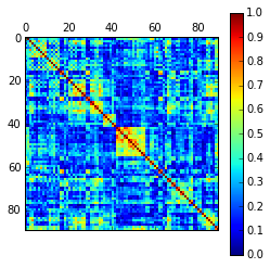
The PLV values for the 90 regions for a particular random subject of our dataset is shown in the next picture:

Which unveils similar structures to the ones got with TE, MI and Correlations.

This week we have been centered in developing new measures for C-PAC. The first one, Transfer Entropy, is related to the first measures we did (Entropy, Mutual Information) addind a lag-time to one of the series, while the second and the third ones have a frequency based approach based on phase synchronization analysys.

Transfer Entropy

The Transfer Entropy has been developed following our interest in measures which would compare past of the signals with his later values (like Granger Causality) and mixing with the Information Theory concept.

Transfer Entropy is a non-parametric statistic measuring the amount of directed (time-asymmetric) transfer of information between two random processes. Transfer entropy from a process X to another process Y is the amount of uncertainty reduced in future values of Y by knowing the past values of X given past values of Y and is denoted as:

1
2
3
4
5
6
7
8
9
10
11
12
13
14
15
16
17
18
19
20
21
22
23

def transfer_entropy(X, Y, lag):
    import numpy as np
    from CPAC.series_mod import cond_entropy
    from CPAC.series_mod import entropy

    # future of i
    Fi = np.roll(X, -lag)
    # past of i
    Pi = X
    # past of j
    Pj = Y

    #Transfer entropy
    Inf_from_Pi_to_Fi = cond_entropy(Fi, Pi)

    #same as cond_entropy(Fi, Pi_Pj)
    Hy = entropy(Pi,Pj)
    Hyx = entropy(Fi,Pj,Pi)
    Inf_from_Pi_Pj_to_Fi = Hyx - Hy

    TE_from_j_to_i = Inf_from_Pi_to_Fi-Inf_from_Pi_Pj_to_Fi

    return TE_from_j_to_i

From this, we have built also a workflow that allows to calculate the TE values over a series of fMRI data. A first test has been carried out with real data using the same dataset of previous entries (a series of 28 subjects and a parcellation of 90 ROIs). Descriptively, mean values over subjects for the TE calculation was reported (left) and connectivity as unweighted was found by thresholding TE values with 0.7 (right).

Phase synchronization and PLV

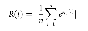
As explained las week, we can obtain the analytical signals using the Hilbert transform. This analytic signal represents a signal in the time domain as a rotating vector with an instantaneous phase, phi(t), and amplitude.

The global level of phase synchrony is given by the parameter R(t), after calculating the modulus of the phase, taking values in the [0,1] range (being 0 completely asynchroneous and 1 completely synchronized, respectively):

Which, translated to python, is:

1
2

def phase_sync(X): # Computes the PS_value as explained in Ponce et al. 2015
#this code is wrong, contact the author

For quantifying the pairwise phase relation between two given brain regions (timeseries) k and l, Phase-Locking Value (PLV) has to be calculated as:

Again, translated to python:

1
2

def PLV(X, Y):
#this code is wrong, contact the author

Some examples with regard of phase synchronization measures will be shown in the next entry of the blog.

This week we have been discussing further about the possibility of developing some frequency analysis tools to integrate in the package. Although CPAC already has some tools to work on the frequency domain, we are thinking in building up some valuable scripts that allow us to capture information using the frequency domain. Our intention is to develop measures such Phase Synchronization and identification of patterns based on frequency domain analysis, to be used as features for Fingerprint analysis. Specifically, as starting point, we are going to take as guide and example the methods described in the paper by Ponce et al. [1], with the intention of performing a similar analysis over fMRI. Our goal is to do so and extending them with measures like temporal power spectral density (PSDT).

Phase synchronization analysis

This kind of analysis needs of the extraction ef the phases of the fMRI timeseries. We can obtain the analytical signals using the Hilbert transform. This analytic signal represents a signal in the time domain as a rotating vector with an instantaneous phase, phi(t), and amplitude.

The global level of phase synchrony is given by the parameter R(t), taking values in the [0,1] range (being 0 completely asynchroneous and 1 completely synchronized, respectively):

For quantifying the pairwise phase relation between two given brain regions (timeseries) k and l, Phase-Locking Value (PLV) has to be calculated as:

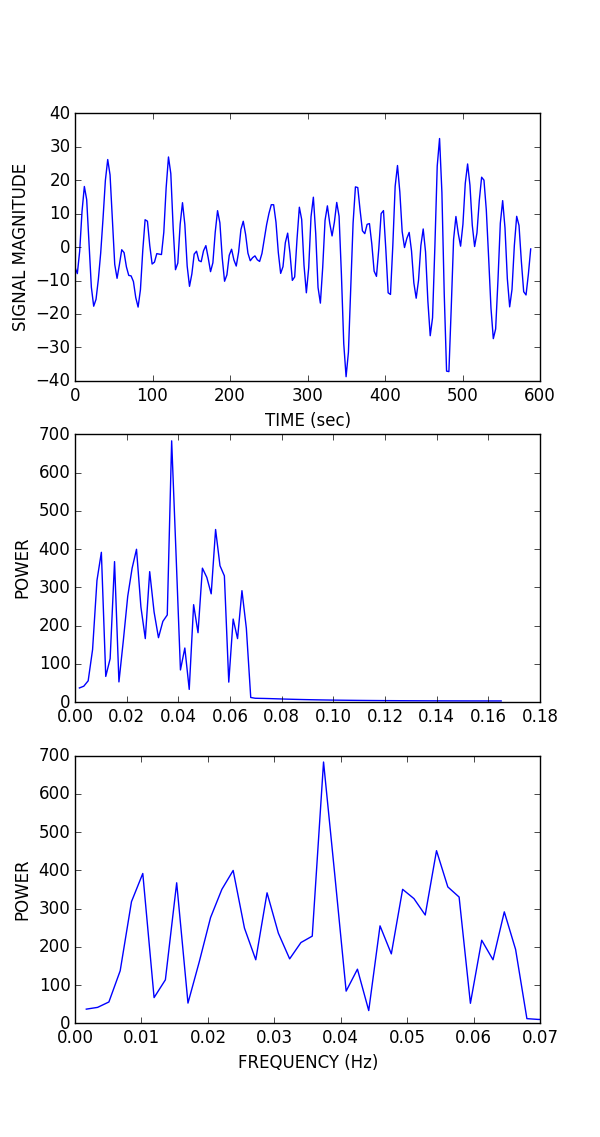
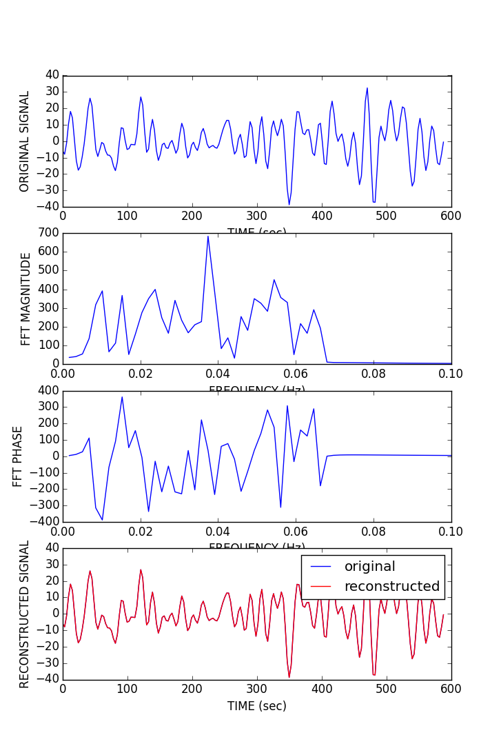
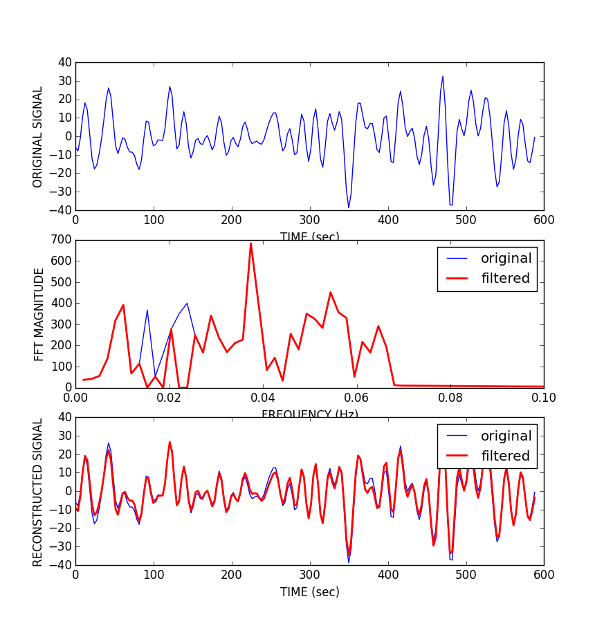
Last week, I already deveveloped a simple filter and this week I have been practicing further with the numpy.signal package. Some example of code, partially changed from this excellent tutorial. Under each block of code, I have plotted an example over fMRI data (it is clear that the used data has been already preprocessed and filtered):

1
2
3
4
5
6
7
8
9
10
11
12
13
14
15
16
17

  from numpy import *
  from scipy import * # not a good practice, but just for the examples

  # Power Spectra calculation
  # construct signal
  t = linspace(0, 1, 1001)
  y = sin(2*pi*t*6) + sin(2*pi*t*10) + sin(2*pi*t*13)

  # compute FFT and the magnitude spectrum
  F = fft.fft(y)
  N = len(t)             # number of samples
  dt = 0.001             # inter-sample time difference
  w = fft.fftfreq(N, dt)     # gives us a list of frequencies for the FFT
  ipos = where(w>0)
  freqs = w[ipos]        # only look at positive frequencies
  mags = abs(F[ipos])    # magnitude spectrum
  phase = imag(F[ipos])  # phase component

1
2
3
4
5
6
7
8
9
10
11
12
13
14
15
16
17

  # Inverse Fast Fourier transform (IFFT) (reconstruction from freq domain)
  # construct signal
  t = linspace(0, 1, 1001)
  y = sin(2*pi*t*6) + sin(2*pi*t*10) + sin(2*pi*t*13)
  
  # compute FFT and the magnitude spectrum
  F = fft.fft(y)
  N = len(t)             # number of samples
  dt = 0.001             # inter-sample time difference
  w = fft.fftfreq(N, dt)     # gives us a list of frequencies for the FFT
  ipos = where(w>0)
  freqs = w[ipos]        # only look at positive frequencies
  mags = abs(F[ipos])    # magnitude component
  phase = imag(F[ipos])  # phase component
  # inverse
  yr = fft.ifft(F)
  

1
2
3
4
5
6
7
8
9
10
11
12
13
14
15
16
17
18
19
20
21
22
23
24
25
26
27
28

  ## Filtering
  # construct signal 
  t = linspace(0, 1, 1001)
  y = sin(2*pi*t*6) + sin(2*pi*t*10) + sin(2*pi*t*13)
  
  # compute FFT and the magnitude spectrum
  F = fft.fft(y)
  N = len(t)             # number of samples
  dt = 0.001             # inter-sample time difference
  w = fft.fftfreq(N, dt)     # gives us a list of frequencies for the FFT
  ipos = where(w>0)
  freqs = w[ipos]        # only look at positive frequencies
  mags = abs(F[ipos])    # magnitude component
  phase = imag(F[ipos])  # phase component
  ip = where(F>5)[0]     # find peaks in FFT
  Fs = copy(F)           # make a copy of the signal FFT
  Fs[ip[[2,3]]] = 0      # set peaks corresponding to 

  yf = fft.ifft(Fs)          # reconstruct
  ip = where(F>5)[0]     # find peaks in FFT
  Ff = copy(F)           # make a copy of the signal FFT
  Ff[ip[[1,2,3,4]]] = 0  # set 10Hz and 13Hz peaks to zero
  magsf = abs(Ff[ipos])  # magnitude component
  phasef = imag(Ff[ipos])# phase component
  yf = fft.ifft(Ff)          # reconstruct
  
  yr = fft.ifft(F)