We are trying to converge to an easy and clear design of the GUI of our toolbox that integrates in CPAC’s structure and allows users to use it. We are trying here to avoid redundant options in the workflow and it is becoming a quite difficult task, since we want the measures to be separated in differentiated subgroups, but at the same time, give the toolbox the possibility of using common functions (such as the extraction of the timeseries). It has to be non-redundant in this way, the most complicated thing will be the correct use of data structures (to take the ones that are already being generated from other modules in CPAC and to check if the series of a volume had been already extracted, in order to do not duplicate efforts). The design has to be generalizable enough that it can be used in other workflows.

Planning of the GUI for NLTSA module

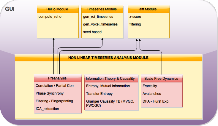
As the most important part of developing new software, it is always necessary to have a good developing plan. For the purpose of building the GUI for our toolbox, we have divided all our measures in 3 main groups:

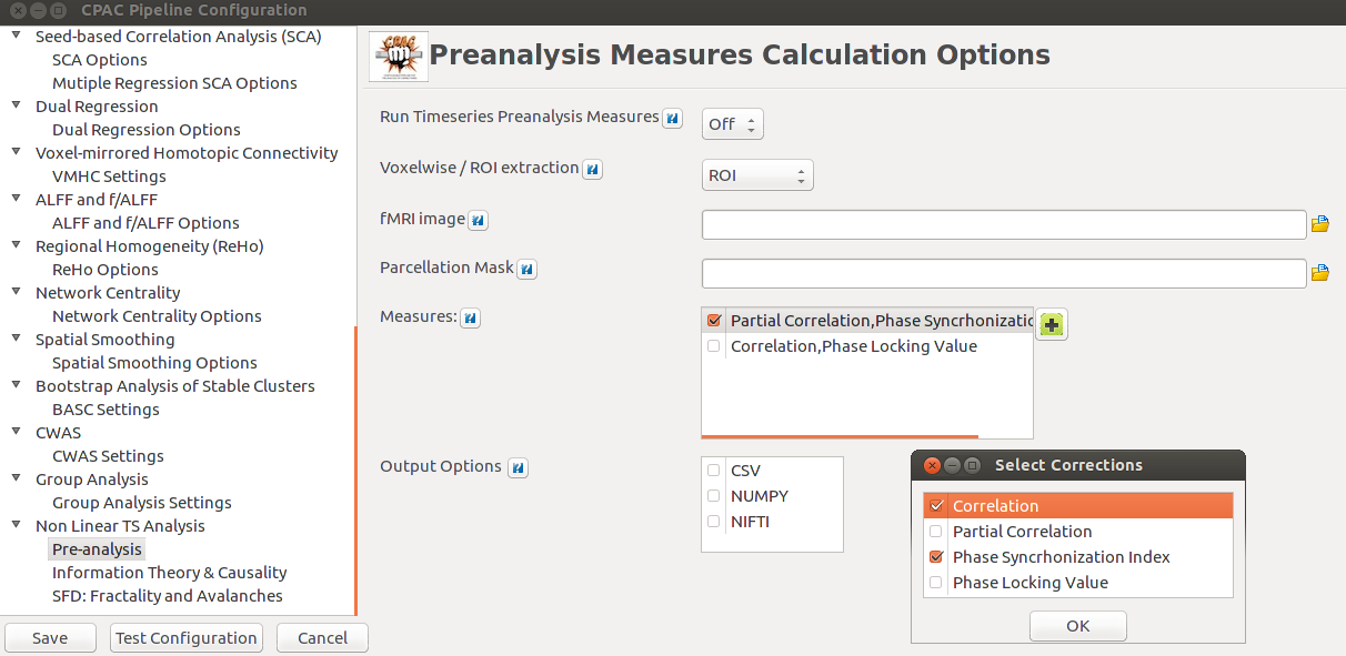
• Pre-Analysis measures: The ones that not correspond directly to NonLinearTimeSeriesAnalysis and can be applied directly into the extracted data. We can find here synchrony measures in time (correlation, partial correlation) and frequency domain (phase synchrony index, phase locking value). Also, treatment of fingerprints and ICA timeseries extraction are due to be added in this submodule.
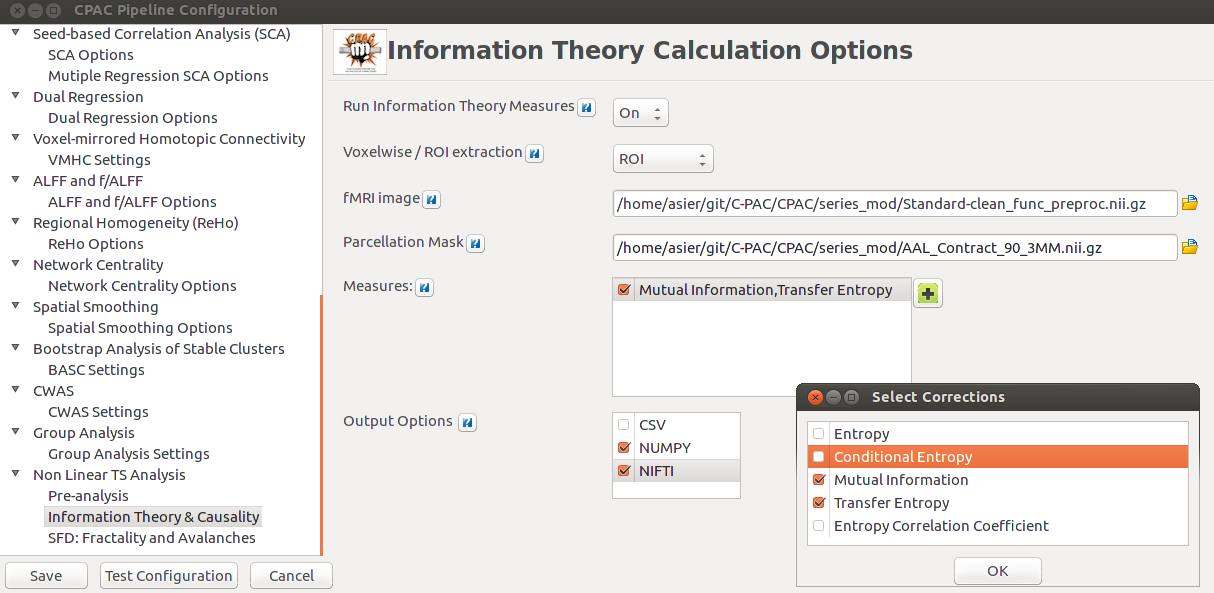
• Information Theory and Causality measures: The ones coming from the informative framework and causality. These measures involve the acquisition of information flow and sharing between variables (Mutual Information, Transfer Entropy, Granger Causality Toolbox measures (MVGC, PWCGC)).
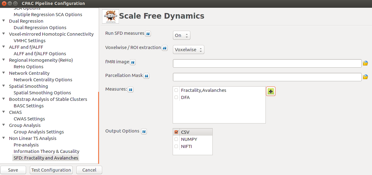
• Scale free dynamics measures: This is the box that make use of the most advanced measures (fractality, avalanches, detrended fluctuation analysis, Hurst exponents). These measures are still pending of being developed (planned for August), so we have still not decided about the inputs and the outputs they are generating.

The schema shown above has been resumed in the next diagram. Most of the modules make use of other modules functions (we have tried to not being redundant with CPAC’s code). We have ensured that the helper functions developed for our toolbox are available also from outside our module.

Implementation of the GUI

Following the instructions published in the previous post, there has been straightforward to build up the 3 subgroups, as they are quite similar between each other. The most important feature for us was the possibility of calculating the measures independently (there is no need of calculating all of them, the user can choose whether to apply the different measures without restriction).

A serious work must be done in flow-controlling inside cpac_pipeline.py to avoid repeating the operations present in the submodules (mainly, timeseries generation. Once that are generated, there is no point in extracting them again). Also, it is important to have well connected the toolbox to the main CPAC’s workflow and check whether the data has been previously extracted. Maybe we can talk at some point soon about this and listen to developers thoughts, comments in the post will be very welcomed. Also, we left the door open for interesting modifications that could happen (the 3rd submodule is still pending of being coded and we have in mind to deal with visualization and data presentation). The whole integration will be held in the last week of GSoC with the help of all collaborators and students.

Synchrony measures in ADHD data

As we are trying not to evaluate all our measures together at the end, this week we have tried extensively our new dataset from ADHD200 (specific information about the dataset and how we did our first experiment in previous post ).

We had two measures to test over this data, “phase synchrony index” (which is a self-informative value about the synchrony level of a specific signal) and “phase locking value” (which is the relation between the synchronicity of 2 variables).

We had two measures to test over this data, “phase synchrony index” or PSI (which is a self-informative value about the synchrony level of a specific signal) and “phase locking value” or PLV (which is the relation between the synchronicity of 2 variables).

Results

The PSI is a single variable measure, so it is just an self-informative measure. First results showed that the data extracted with the cc400 and cc1000 parcellations had a low synchrony level (some of them looked totally desynchronized). Overall, there was not much to say about differences between ADHD patients and controls.

The PLV, however, showed that the synchrony between some of the signals was strong (>0.7). As these parcellations are randomly created and assigned, consecutive ROIs have not spatial relation and showing the usual matrixes was not going to be informative.

Solved GC VAR model calculation

We have changed the paradigm of measuring the residuals for the Granger Causality calculation. Instead of calculating the covariance matrix of the data, which was creating problems later with the VAR model, we have change this. Now, the residuals are calculated directly from the data (the regression model used was OLS using QR decomposition. Specifications in MVGC toolbox docs), without performing the calculation of the covariance matrix.

We performed a small evaluation of the PWGC over our ADHD200 dataset and results were not visually different between groups. We are working in an appropriate way of showing results coming from these measures.