This week we have been centered in developing new measures for C-PAC. The first one, Transfer Entropy, is related to the first measures we did (Entropy, Mutual Information) addind a lag-time to one of the series, while the second and the third ones have a frequency based approach based on phase synchronization analysys.

Transfer Entropy

The Transfer Entropy has been developed following our interest in measures which would compare past of the signals with his later values (like Granger Causality) and mixing with the Information Theory concept.

Transfer Entropy is a non-parametric statistic measuring the amount of directed (time-asymmetric) transfer of information between two random processes. Transfer entropy from a process X to another process Y is the amount of uncertainty reduced in future values of Y by knowing the past values of X given past values of Y and is denoted as:

1
2
3
4
5
6
7
8
9
10
11
12
13
14
15
16
17
18
19
20
21
22
23

def transfer_entropy(X, Y, lag):
    import numpy as np
    from CPAC.series_mod import cond_entropy
    from CPAC.series_mod import entropy

    # future of i
    Fi = np.roll(X, -lag)
    # past of i
    Pi = X
    # past of j
    Pj = Y

    #Transfer entropy
    Inf_from_Pi_to_Fi = cond_entropy(Fi, Pi)

    #same as cond_entropy(Fi, Pi_Pj)
    Hy = entropy(Pi,Pj)
    Hyx = entropy(Fi,Pj,Pi)
    Inf_from_Pi_Pj_to_Fi = Hyx - Hy

    TE_from_j_to_i = Inf_from_Pi_to_Fi-Inf_from_Pi_Pj_to_Fi

    return TE_from_j_to_i

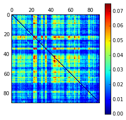
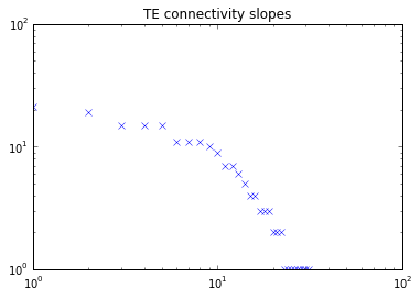
From this, we have built also a workflow that allows to calculate the TE values over a series of fMRI data. A first test has been carried out with real data using the same dataset of previous entries (a series of 28 subjects and a parcellation of 90 ROIs). Descriptively, mean values over subjects for the TE calculation was reported (left) and connectivity as unweighted was found by thresholding TE values with 0.7 (right).

Phase synchronization and PLV

As explained las week, we can obtain the analytical signals using the Hilbert transform. This analytic signal represents a signal in the time domain as a rotating vector with an instantaneous phase, phi(t), and amplitude.

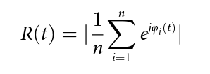
The global level of phase synchrony is given by the parameter R(t), after calculating the modulus of the phase, taking values in the [0,1] range (being 0 completely asynchroneous and 1 completely synchronized, respectively):

Which, translated to python, is:

1
2

def phase_sync(X): # Computes the PS_value as explained in Ponce et al. 2015
#this code is wrong, contact the author

For quantifying the pairwise phase relation between two given brain regions (timeseries) k and l, Phase-Locking Value (PLV) has to be calculated as:

Again, translated to python:

1
2

def PLV(X, Y):
#this code is wrong, contact the author

Some examples with regard of phase synchronization measures will be shown in the next entry of the blog.