The Hilbert Transform is a linear operator which takes a function, u(t), and produces a function, H(u)(t), with the same domain.

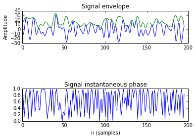
In python, we can compute the analytic signal, using the Hilbert transform. This analytic signal is used for many things, like computing the envelope of a signal or the instantaneous phase of the signal. Our calculation of the instantaneous phase is in the range [0,1], computed over the cos() function of the angle of the Hilbert Transform coefficients. We have choosen a random signal of an fMRI file to show the example:

1

env = numpy.abs(sigtool.hilbert(s))

1
2
3

ht = sigtool.hilbert(s)
px = np.angle(ht) # instantaneous phase
inst_p = np.sqrt((np.cos(px))**2) # modulus of the angle in [0,1]

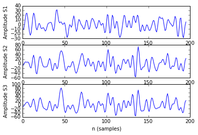
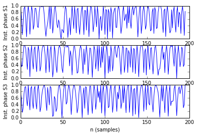
With this instantaneous phase, we can code easyly the two functions that were shown in the previous post, the Phase Synchronization parameter and the Phase Locking Value. For visualization purposes, here is shown a good example of three signals, the first one is from a region far from the other ones. The last two signals are in regions close to another (it is supposed they will be more synchronized between them than with the first one, which is distant).

The PLV values, validating our initial hypothesis, are the following:

• PLV(S1,S2) = 0.43
• PLV(S1,S3) = 0.41
• PLV(S2,S3) = 0.86

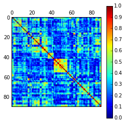
The PLV values for the 90 regions for a particular random subject of our dataset is shown in the next picture:

Which unveils similar structures to the ones got with TE, MI and Correlations.