Last week we dealt with some aspects on how to construct the workflows:

• Develop fully functional ones where to integrate functions. ✓ [Currently, to make transformations with the data generated during the workflow, you have to specifically save it]

1

   np.savetxt(in_file+'_corr.txt', corr_mat)

• Test and validate in a pilot real data over the workflows and see if we can get some interesting results. ✓ [it has been done using different type of data (filtered, non-filtered…), different measures (corr, pcorr and MI) and, in the case of MI, different bin(states) numbers (see 2nd part of the post)]
• Implement further synchronization analysis measures. ✓ [partialcorr workflow was studied and added to the package and Entropy Correlation Coefficient was implemented as in [1]. Also, it was studied the lossless dimensional discretization by the use of better optimal discretization, sampled entropies and recurrence statistics.

Testing workflows with real data

I’ve tested the Correlation (corr), Partial Correlation (pcorr) and Mutual Information (MI) with 3 different bin_number: 20, 50 and 100, as a pilot approach, were as proper optimization and framework is being fully developed aside. Workflow was tested throughs a dataset of 29 subjects (196 timepoints*voxel) and a 90 ROI parcellation mask (another mask with more parcellations was used, see below). The data was preprocessed and filtered (no global signal was regressed), and rest of criteria were the standards as in [2]. I’ve printed some graphs to comment on results:

a) Randomly selected one matrix (one subject) of each one of the measures: corr, pcorr and MI20 (MI50 and MI100 were too sparse, see below). Corr and MI captured some structures (most of them in common) and pcorr was not able to. We are going to try to figure out what happened with pcorr and if this is a suitable result for this measure. In the other hand, results were quite robust between subjects, unveiling similar relations between ROIs. See below the mean matrix over subjects.

b) Connectivity as unweighted was found by thresholding correlations with 0.7.

c) Descriptively, mean values over subjects for MI20, MI50 and MI100. The principal diagonal was set to 0 for visualization purposes, as these values represent the Entropy and are higher that the rest. As can be seen, the reported structures change with the amount of bins chosen. Having a very blurry effect in MI100 and structures better defined in MI20 (more small MI values, but structures better captured). This is mainly because having 100 states for a signal with 196 timepoints, reduces the possibility of repeating a state, thus, the maximum value of the MI increases (approximating the maximum possible Entropy) as the number of bins increases.

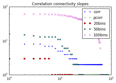
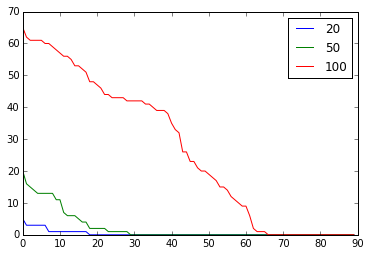
If we superpose again the sorted frequencies in the matrices, using those 3 prospective thresholds, we obtain a similar pattern of also acceptable information lossless discretization. However, the choice of threshold was something more arbitrary that we had not been able to discuss.

Theory and discussion

We also progressed in discussion, I’ve a clearer vision of how to implement Multivariate Conditional Granger Causality, based on the one in [3] , implementing “conditional” Granger Causality in multivariate manner [4]. For this purpose, we will program an algorithm that uses the autocovariance sequence and discover whether one of these sequences is reducing the uncertainty of the second (with the mean prediction error), having into account the rest of the series. The order of the model will be likely to be 1, since the TR has a low frequency and the dynamics between the source and the target for order higher would be too separated from each other. The implementation is still in research phase, but I’ve done some experiments with randomly generated series:

1
2
3
4
5

X = np.random.randn(1000)
Y = np.random.randn(1000)

Z = Y.copy();
Z[1:] = Z[1:] + X[0:-1] #so: X influences Z with timelag 1 (order)

And then, as explained here.

With this, we are heading towards a transition from the first to the second box of measures that we were thinking of (the first one more related to preprocessing like filtering, synchronization, basic entropies… and the second one as an analysis module, where we are adding Conditional Granger Causality, Mutual Information, Entropy Correlation Coefficient and many more to come). Anyway, we are not closing the door of the first box, since we have in mind to implement surrogate analysis as in [5] to unveil non-linear phenomena occurring.

Moreover, we were thinking in implementing some kind of preprocessing scripts for frequency-filtering and computing the z-score of the series. Actually, an easy band_pass filter was added to the repo . But then we realised that CPAC already has this functionality implemented, it works fine and there is no point in duplicating it. We will save the bp filter in case we want to use it later on, as we have seen that could be interesting to save some specific bandwidth for some analyses [6]. We will further discuss these options, as we are heading towards frequency and coherence analysis as we see that it will bring us interesting possibilities.