This week, as planned from the previous one, the integration has been extensively worked: the cpac_pipeline.py has now our workflow fully integrated and I have change the workflows into a single one, making it easier the call to the methods. Also, the treatment of the inputs has changed, since we are not making the extraction of the series anymore (another module of C-PAC is taking the responsibility). But more interestingly, we have enforced the Criticality package with the correction of the Point Process and Conditional Rate Mapping from the previous week and the developing of 2 new functions: Clustering and Avalanche detection algorithms.
For this algorithms, we have also followed the headlines explained in the paper of Tagliazucchi et al (“Criticality in large-scale brain fMRI dynamics unveiled by a novel point process analysis”), we have been able to extract Avalanches in the brain, wich opens a new perspective in the analysis of brain dynamics in C-PAC.
Clustering Detection
The technique is described, extracted from the section Methods of the paper, as:
To detect contiguous clusters of activated voxels (defined as those crossing the threshold), for each time step, the problem was reduced to the detection of connected components in a suitably defined graph or network. More precisely, for each volume, a graph was constructed having each voxel as a node, and two nodes connected with a link if they were both activated (BOLD signal above 1 SD) and also first neighbors in the spatial sense. The connected components of this graph correspond to clusters of contiguous activated voxels isolated from other similarly defined clusters.
The implementation of this approach was straightforward, but it has many checks to do, so it is an algorithm to code very carefully. It is a first draft of the algorithm and the purpose was to have a functional procedure asap. In future revisions, I will try to rewrite it in a more “pythonic way”.
1 2 3 4 5 6 7 8 9 10 11 12 13 14 15 16 17 18 19 20 21 22 23 24 25 26 27 28 29 30 31 32 33 34 35 36 37 38 39 40 41 42 43 44 45 46 47 48 49 50 51 52 53 54 55 56 57 58 59 60 61 62 63 64 65 66 67 68 69 70 71 72 73 74 75 76 77 78 79 80 | |
Avalanche Detection
The technique can be easily described, extracted from the section Methods of the paper:
The point process is defined by the sequences of time points at which the BOLD signal crosses a given threshold from below. (…) To construct the conditional rates the point process is defined at a seed location and at the targets throughout the entire brain. The BOLD signal is extracted from a seed region (top trace) and the points (arrows and vertical dashed lines) are defined by the crossings at 1 SD (horizontal dashed lines). Every time the signal at a target region crosses the threshold (asterisks) up to 2 time steps later than in the seed, the rate at the target is increased in one unit. This rate is normalized by the number of points in the seed. The top panel shows the location of the seed and of the two example targets, as well as the resulting average conditional rates maps (left) and DMN obtained from PICA (right). Medium panels show the BOLD signal at the seed and at the two example target regions.
1 2 3 4 5 6 7 8 9 10 11 12 13 14 15 16 17 18 19 20 21 22 23 24 25 26 27 28 29 30 31 32 33 34 35 36 37 38 39 40 41 42 43 44 45 46 47 48 49 50 51 52 53 54 55 56 57 58 59 60 61 62 63 64 65 66 67 68 69 70 71 72 73 74 75 76 77 78 79 | |
Discussions on Clustering and Avalanche detection
Clustering Detection
After coding the algorithms as explained in the paper, we extended it to some discussion, we found further questions of interest with regard to the algorithm. Questions that have emerged after initial implementation are the following:
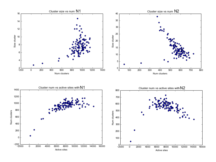
I was wondering about the root aspects of defining 1 single neighbour and not more in the clustering detection and also about the decision of determining a cluster just from one neighbouring. Which are the implications of these assumptions? I actually tried the implementation extending the neighbouring adding more neighbours (2 and 3).
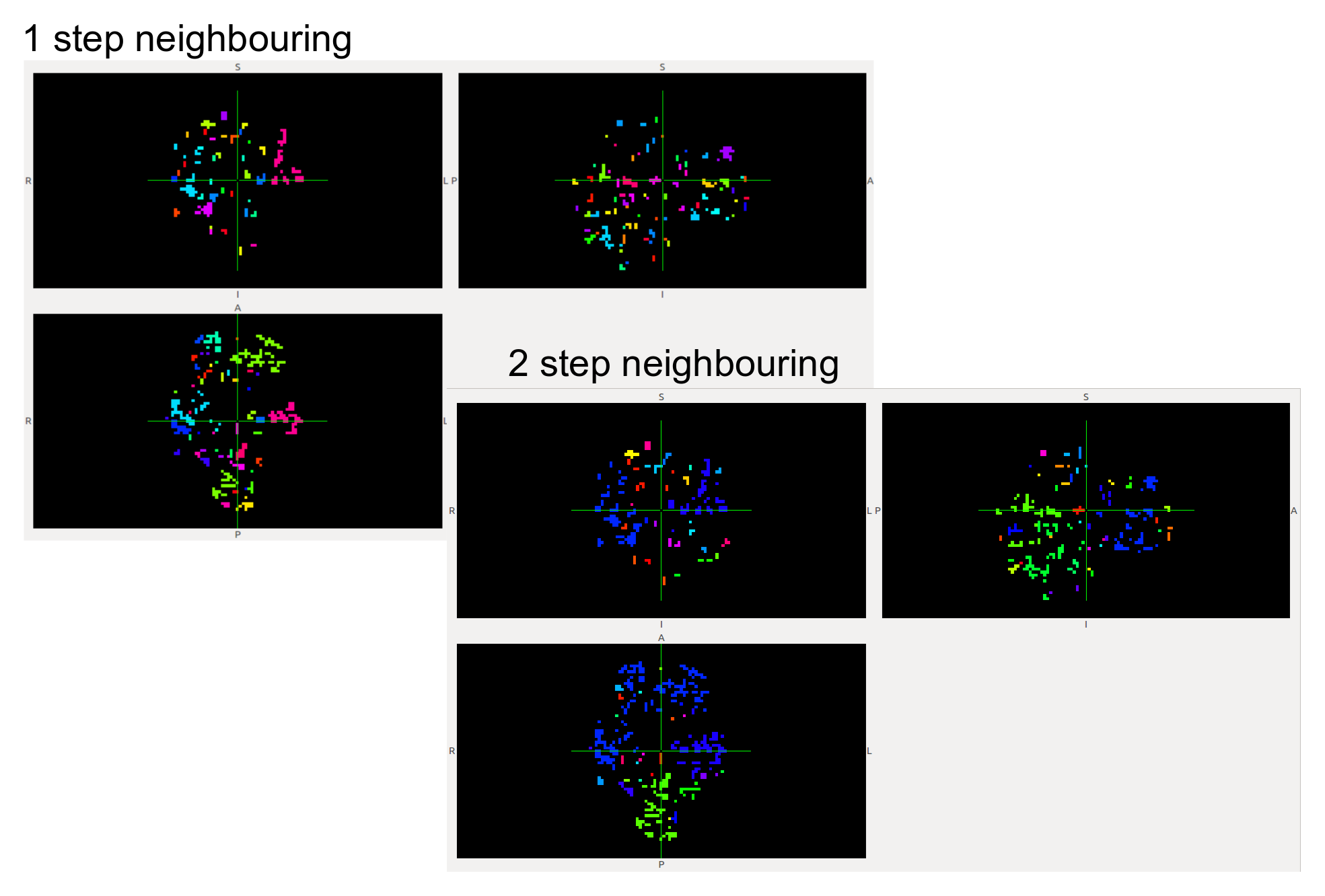
I came across with less and bigger clusters, which we discussed for its possible interest specifically with brain images. See images below for clusters with the proposed 1 distance for neighbours and with a distance of 2, at a given time:

From these approaches we can have some statistics, showing that the choice of the number of neighbours to consider is not a trivial decision:

Avalanche Detection
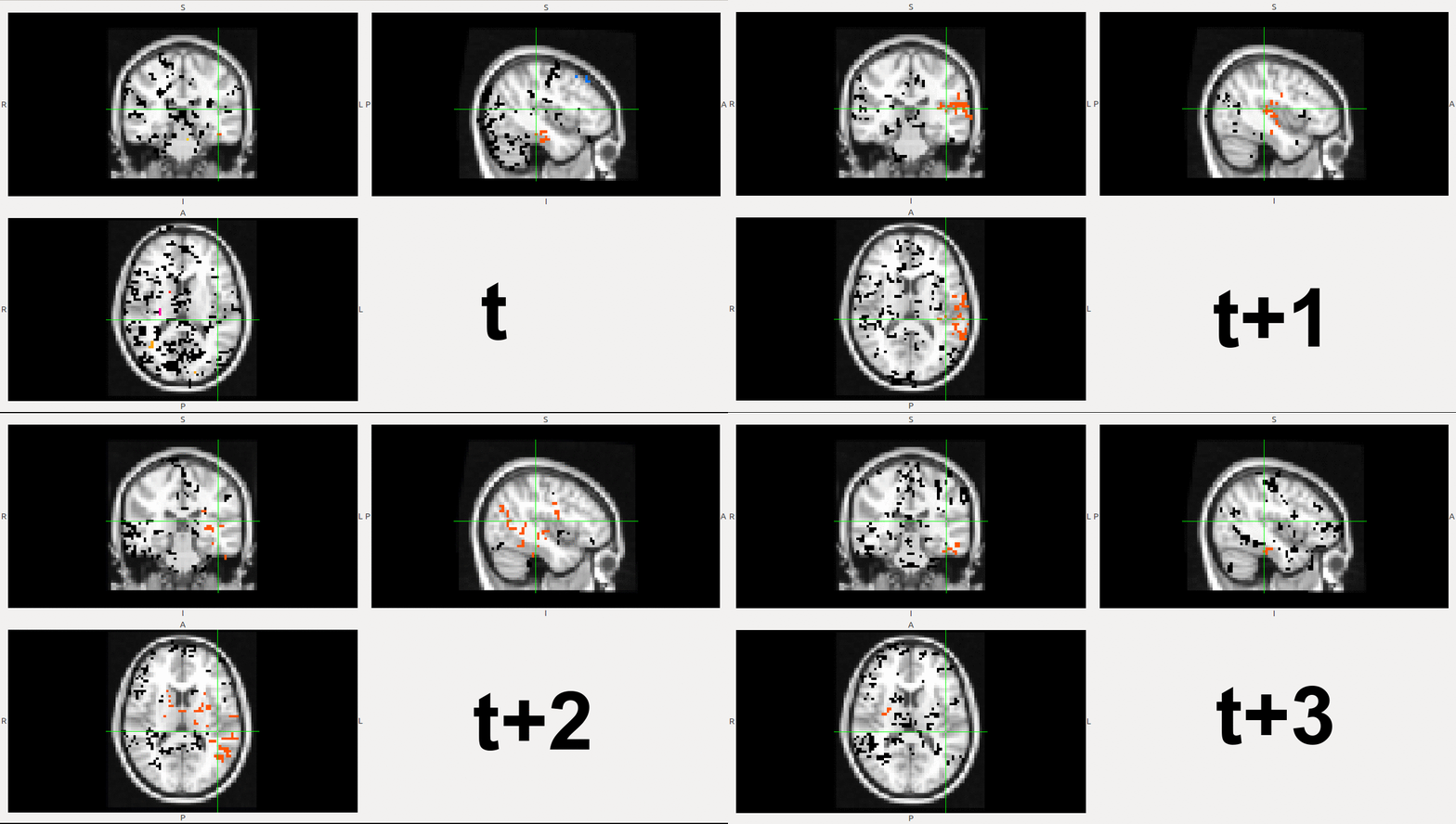
We collected all the avalanches for a given subject in a 4D Nifti file. Avalanches were significantly different depending of the choice of the neighbouring size (due to the change of the size of the mean cluster). Here we show a first approximation, we would have liked to make a movie, but we ran out of time for this week.

Here I have made a gif to represent how an avalanche is. This is an avalanche for the N2 cluster, take into account just the voxels in red/orange. It can be showed how the avalanche borns, grows and spreads, and finally dies.
Heading last week of coding
Our objectives for next week are:
Perform extensive testing over the measures and chose which ones are going to be in the package.
Make code corrections and comment all the measures. This will head us into the documentation we have to make.