We are heading the end of the quarter and our toolbox is starting to be mature, while we investigate the many links and uses between tools. This week we have gone through important steps (but at the same time ongoing discussions due to the rich materials produced at this stage). Two main new things we have done, beyond the polishing of previous tools and validating ongoing:

• The integration of the toolbox in CPAC’s pipeline is almost complete. This has been a tough task to do, since the internals of CPAC are quite large, with many flows and structures, but the main idea is clear: The work to do is to link the inputs you get from the GUI and the data already calculated previously in other CPAC’s modules with your workflows inputs and integrate them in the main pipeline.

• Point Process Analysis and Conditional Rate Maps calculation: Following the initial plan, we have developed some new methods to test the time scale side of the toolbox and while Supraja is progressing with multifractal analysis in parallel.

Following the instructions in the paper of Tagliazucchi et al (“Criticality in large-scale brain fMRI dynamics unveiled by a novel point process analysis”), we have been able to code the base point process approach followed of a Conditional Rate Map building as in the paper.

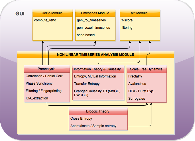
And last, in terms of toolbox integration, new cross relationships have been looked at. Some of those are portrayed from our last model:

Integration of the toolbox in CPAC’s pipeline

After carefully having explored the main pipeline, we realized that in order to not to repeat code and structures that are already developed, I had to make some changes in my initial workflows. At the beginning of the project, I coded them as independent workflows, with independent behaviour and inputs, and some helper functions that are already integrated in CPAC but that where necessary for me in that moment. Now, I have to link the data that would be already in CPAC, change the treatment of the inputs of my workflows and integrate them as a single tool.

That will have effect too in the configuration of the GUI I proposed two weeks ago, being now more efficient. We have now all measures in a joint page of the GUI, having separated each of the main boxes of the initial plan in three different checkboxes with a common input. Also, the input data for my workflows will come from the TSE module of CPAC, which already makes these extractions. I have to modify my functions to work with 1D files (I have already the main code block built, since I already treated with this data type in the analysis of the 400 regions).

In the main pipeline, I have inserted the NLTSA workflow:

https://github.com/roijo/C-PAC_complexitytools/blob/master/CPAC/pipeline/cpac_pipeline.py#L3207-L3368

It can be seen in the code that still are many things to change and improve, I am receiving crucial help from developers, to fully understand how the main pipeline works and transferring this knowledge to all discussions.

The main structure at the moment, is a three block structure as previously proposed, plus the insert of qualities that measures derived from ergodic theory rely on. From these, I let the user to choose which one of them (the measures inside each of them) to calculate. I will change my workflows (I will have one per measure-box) and inside them, the measures will be called directly depending if they have been chosen by the user or not.

Point Process Analysis and Conditional Rate Maps

The technique can be easily described, extracted from the section Methods of the paper:

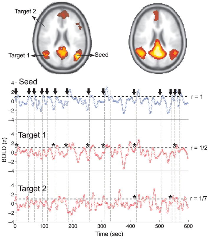
The point process is defined by the sequences of time points at which the BOLD signal crosses a given threshold from below. (…) To construct the conditional rates the point process is defined at a seed location and at the targets throughout the entire brain. The BOLD signal is extracted from a seed region (top trace) and the points (arrows and vertical dashed lines) are defined by the crossings at 1 SD (horizontal dashed lines). Every time the signal at a target region crosses the threshold (asterisks) up to 2 time steps later than in the seed, the rate at the target is increased in one unit. This rate is normalized by the number of points in the seed. The top panel shows the location of the seed and of the two example targets, as well as the resulting average conditional rates maps (left) and DMN obtained from PICA (right). Medium panels show the BOLD signal at the seed and at the two example target regions.

From that explanation a pair of functions have been developed:

1
2
3
4
5
6
7
8
9
10
11
12

# Point process analysis for a signal. Values equal to 1 when the original value 
# is higher than the threshold (1*SD)
def point_process(signal):

    import numpy as np

    pp_signal = np.zeros(signal.shape[0])
    th = np.std(signal)

    pp_signal[signal > th] = 1

    return pp_signal

1
2
3
4
5
6
7
8
9
10
11
12
13
14
15
16
17
18
19
20
21
22
23
24
25
26
27
28
29
30
31
32
33
34
35
36

# Conditional Rate Map. Given an fMRI, extract timeseries, calculate Point Process
# and then the Rate Map for each voxel given a seed   
def cond_rm(in_file, seed_location):

    import numpy as np
    import os
    import nibabel as nb

    # Treat fMRI image
    img = nb.load(in_file)
    #print img.shape
    data = img.get_data()

    (n_x, n_y, n_z, n_t) = data.shape

    K = np.zeros((n_x, n_y, n_z))
    # Extract seed and pp
    seed_data = data[seed_location[0], seed_location[1], seed_location[2],:]
    pp_seed_data = point_process(seed_data)
    r = np.count_nonzero(pp_seed_data)
    # Calculate each PP signal
    for i_ in range(n_x):
        for j_ in range(n_y):
            for k_ in range(n_z):

                target_data = data[i_,j_,k_,:]
                pp_target_data = point_process(target_data)

                # LOGIC AND (target/seed) and count(signal == 1), that will give you the X/r parameter [0,1]
                K[i_,j_,k_] = np.count_nonzero(np.logical_and(pp_seed_data,pp_target_data))/float(r)

    # Reconstruct the 3D volume
    cond_rm_file = os.path.join(os.getcwd(), 'cond_rm.nii.gz')
    img.to_filename(cond_rm_file)

    return cond_rm_file

As it can be seen, there is still a small change to be done in the CRM function. As described in the paper, the target point processed signal has to be checked in the same time point as the seed and up to 2 time steps later. As it can be derived from the image, is takes all the values crossing the threshold in a row just as one crossing. I would like to keep my function in a pythonic way and I don’t find a way of computing the CRM without messing everything up with index checking to satisfy the requirements of the algorithm. Also, it would be desirable to know if the data already satisfies the requirements of z-scoring and HRF deconvolution as proposed in the paper and if this has effect on the algorithm results.

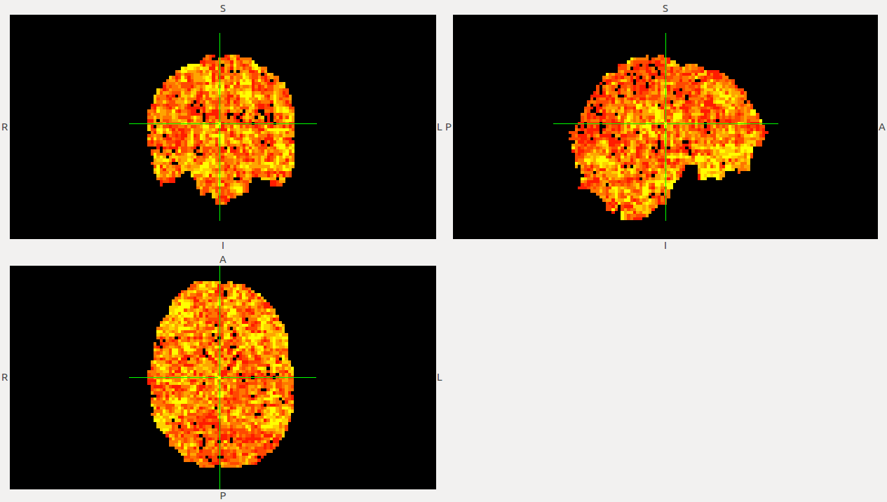
From these calculations, we can start extracting volumes such as:

We are now discussing about the possibility of following the analysis by building the Clustering and the Avalanche detection, but they are not as well described in the paper and we have to make a evaluation of the time we have to finish the project.

Relation between Correlation and CMR’s number of point-wise events

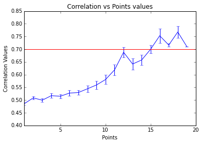
To make a comparison between the number of points that are necessary to reach a specific information level with the point process algorithm, we have used the correlation to identify highly synchronized timeseries. What we have done here is to build a relation between the synchrony of two variables and the point peaks that share each other after point processing them (CMR without normalizing).

As an initial optimization we can find to which level point process transients can be translated to a point of criticality. This analysis has been produced at the voxel-wise level from ABIDE subjects, properly checked and preprocessed. Here, we can see how the increasing of the (mean) synchrony between two variables, increases the points that they share. This is a really nice finding, because it shows how point process can describe the change of regime associated with functional connectivity.

We can observe how once reached a threshold of 0.7 correlation point-processes can saturate giving a new quality to connectivity between regions.

Others

• Even if the VAR model calculation was corrected in the previous week, there was still an issue with the calculation of pwcgc() , the internal loop has been already corrected. We have tested the function over data and looks to have the same performance as the original Matlab function. Different distributions of these will be last discussed if we can define more optimal models.

• We have been discussing about the need of visualization of some analysis inside and some statistics CPAC (Pandas integration) . This is maybe a sore point that would be better to discuss with main developers.

• Next week we will follow our work with the integration, enforcement of criticality package and also we are into final integration of all our measures (phase measures integration with Scale Free Dynamics ones like DFA/Hurst exponent, for example).