BUILDING NON-LINEAR ANALYSIS TOOLS FOR C-PAC

Contributing to C-PAC

Multivariate Granger Causality in Python for fMRI Timeseries Analysis

Wiener-Granger causality (“G-causality”) is a statistical notion of causality applicable to time series data, whereby cause precedes, and helps predict, effect. For the purpose of analysing fMRI timeseries, we have developed as a first approach a series of python scripts to calculate the Multivariate Granger Causality (MVGC) based on the MVGC toolbox of Barnett & Seth [1]. The most common operationalisation of G-causality, and the one on which the MVGC Toolbox is based, utilises VAR (vector autoregression) modelling of time series data. But it is not the only one, and our intention is to explore other options too and extend to other options that could be more robust.

G-causality assumes two jointly distributed vector-valued stochastic processes (“variables”) X = X1 , X2 , …, Y = Y1 , Y2 , …. We say that X does not G-cause Y if and only if Y, conditional on its own past, is independent of the past of X; intuitively, past values of X yield no information about the current value of Y beyond information already contained in the past of Y itself. If, conversely, the past of X does convey information about the future of Y above and beyond all information contained in the past of Y then we say that X G-causes Y, as you can see in the image.
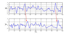
image

The steps to calculate MVGC are the following: We first have to compute the autocovariance matrix from the timeseries. After that, extract the coefficients with the VAR modelling and finally, perform the calculation of the MVGC. More detailed explanations and comments of the code on GitHub and the paper itself. In the following example, X is the timeseries matrix and q is the order of the model (number of lags).

1
2
3
4
5
6
7
8
9
10
11
12
13
14
15
16
17
def tsdata_to_autocov(X, q):

    import numpy as np
    from matplotlib import pylab

    if len(X.shape) == 2:
        X = np.expand_dims(X, axis=2)
        [n, m, N] = np.shape(X)
    else:
        [n, m, N] = np.shape(X)
    X = pylab.demean(X, axis=1)
    G = np.zeros((n, n, (q+1)))

    for k in range(q+1):
        M = N * (m-k)
        G[:,:,k] = np.dot(np.reshape(X[:,k:m,:], (n, M)), np.reshape(X[:,0:m-k,:], (n, M)).conj().T) / M-1
    return G

For the calculation of the MVGC, inputs needed are G (autocovariance sequence), x (vector of indices of target (causee) multi-variable) and y (vector of indices of source (causal) multi-variable). The MVGC calculation, extracts the coefficients with the VAR model of all variables (x, y, z) and then without the source (x,z). The output F is the Granger Causality itself.

1
2
3
4
5
6
7
8
9
10
11
12
13
14
15
16
17
18
19
20
21
22
23
24
25
26
def autocov_to_mvgc(G, x, y):

    import numpy as np
    from mvgc import autocov_to_var
  
    n = G.shape[0]

    z = np.arange(n)
    z = np.delete(z,[np.array(np.hstack((x, y)))])
    # indices of other variables (to condition out)
    xz = np.array(np.hstack((x, z)))
    xzy = np.array(np.hstack((xz, y)))
    F = 0

    # full regression
    ixgrid1 = np.ix_(xzy,xzy)
    [AF,SIG] = autocov_to_var(G[ixgrid1])

    # reduced regression
    ixgrid2 = np.ix_(xz,xz)
    [AF,SIGR] = autocov_to_var(G[ixgrid2])


    ixgrid3 = np.ix_(x,x)
    F = np.log(np.linalg.det(SIGR[ixgrid3]))-np.log(np.linalg.det(SIG[ixgrid3]))
    return F

To calculate the coefficients:

1
2
3
4
5
6
7
8
9
10
11
12
13
14
15
16
17
18
19
20
21
22
23
24
25
26
27
28
29
30
31
32
33
34
35
36
37
38
39
40
41
42
43
44
45
46
47
48
49
50
51
def autocov_to_var(G):

    import numpy as np

    [n,m,q1] = G.shape;
    q = q1 - 1
    qn = q * n
    G0 = G[:,:,0]
    # covariance
    GF = np.reshape(G[:,:,1:], (n, qn)).T
    # backward autocov sequence
    GB = np.reshape(np.transpose(G[:,:,1:], (0, 2, 1)), (qn, n))

    # forward  coefficients
    AF = np.zeros([n, qn])
    # backward coefficients (reversed compared with Whittle's treatment)
    AB = np.zeros([n, qn])

    # initialise recursion
    k = 1 # model order
    r = q-k
    kf = np.arange(k*n)
    # forward  indices
    kb = np.arange(r*n, qn)
    # backward indices
    AF[:,kf] = np.dot(GB[kb,:],np.linalg.inv(G0))
    AB[:,kb] = np.dot(GF[kf,:],np.linalg.inv(G0))

    for k in np.arange(2, q+1):

        DF = GB[(r-1)*n+1:r*n,:] - np.dot(AF[:,kf],GB[kb,:])
        VB = G0 - np.dot(AB[:,kb],GB[kb,:])

        AAF = np.dot(DF,np.linalg.inv(VB)); # DF/VB

        DB = GF[(k-1)*n+1:k*n,:] - np.dot(AB[:,kb],GF[kf,:])
        VF = np.dot(G0-AF[:,kf],GF[kf,:])

        AAB = np.dot(DB,np.linalg.inv(VF)); # DB/VF

        AFPREV = AF[:,kf-1]
        ABPREV = AB[:,kb-1]
        r = q-k
        kf = np.arange(1, (np.dot(k, n))+1)
        kb = np.arange(np.dot(r, n)+1, (qn)+1)
        AF[:,kf-1] = np.array(np.hstack((AFPREV-np.dot(AAF, ABPREV), AAF)))
        AB[:,kb-1] = np.array(np.hstack((AAB, ABPREV-np.dot(AAB, AFPREV))))

    SIG = G0-np.dot(AF, GF)
    AF = np.reshape(AF, (n, n, q))
    return [AF, SIG]

This is a preliminary version of the MVGC, we now need to test and validate in real data over the workflows and see if we can get some interesting results. Also, we have agreed that it would be useful to code the Pairwise Conditional Granger Causality (which was maybe the first step to make, before MVGC).

Comments